Chapter 19
Measuring
Treatment
Merle Canfield
During the past 50 years there
has been a steady increase in the number of schools or styles of psychotherapy.
In 1984 Karasu, T., et. al. reported 418 systems. At the same time there has been a moderate
increase in the elements of psychotherapy.
In recent years there has been a trend to merge these systems with
common factors. It is the purpose of
this section to show how research designs empirically support the process of
sorting out the characteristics of these system. At the same time the designs should support
the further elaboration and search for the elements of psychotherapy. Frank (1971) proposed that there were common
factors in addition to specific factors in psychotherapy that might be related
to outcome (see also Parloff, 1986).
In an attempt to determine
whether the treatment has been implemented three approaches have been used: (1)
developing therapy manuals, (2) labeling or coding psychotherapy as it unfolds,
and (3) rating the process by the use of scales. In 1979 Russell and Stiles reviewed the
coding systems and attempted to devise a taxonomy and resulting coding system
that would include all elements of the existing coding systems. They generated a logical or rational
taxonomy. Although their task was
different they did attempt do develop a taxonomy of the psychotherapeutic
elements. Many of the taxonomies that
have been developed have been developed for specific style of school of
therapy. We are proposing methods to
perform empirical taxonomies, or a combination of judgments and empirical
These methods can be used in to
ways: (1) develop a taxonomy of the styles of therapy, or (2) develop a
taxonomy of the elements of therapy.
Probably both of these would be useful.
If both were developed they would complement each other so that
identifying a particular style or school of therapy would be a matter of
selecting a set of elements of therapy.
The techniques are similar for the two areas. Finally, modes other than psychotherapy are
presented.
For example, of the 400
different schools what is the overlap and how would one determine the overlap
between the schools? It would be useful
to identify the overlap or common factors.
What are the interactions that
would place a therapeutic interaction within a specific school and separate the
interaction from other schools (unique factors)? What therapeutic interactions overlap with
other schools (common factors). There
are two major tasks to be accomplished if one is to make such
discriminations. The first task is to be
able to identify and measure (either by counting or by assessing some degree)
of the client/therapist interactions. If
that can be accomplished the second task is to indicate the taxonomy of
performances that each of the styles need.
That is, a profile of the style in terms of the performances is needed.
The most fruitful method of identifying these performances has been to code the
utterances of the psychotherapy process.
There are four statistical
methods that might be used for this process: (1) cluster analysis, (2)
discriminant function analysis, (3) multidimensional scaling, and (4) factor
analysis. Four basic therapy processes
discussed are: (1) psychotherapy, (2) group therapy, (3) ancillary therapies,
and (3) milieu therapy. The literature
indicates that the descriptive or taxonomy process has be accomplished most the
psychotherapy, next with group therapy, next the ancillary therapies and
finally milieu is the least identified.
Trochim (19--) and
_______________ used a combination of cluster analysis and multidimensional
scaling to develop maps of attitudes of toward organizations. It is proposed here that the same method
could be used to build a taxonomy of the elements of psychotherapy.
In this example participants were asked to identify processes or
characteristics of psychotherapy that they thought were curative. The following is that list (along with an abbreviated
name):
Develop
insight INSIGHT
desensitize DESENS
reflect REFLECT
introspection INTROSP
develop trust DEVTRUST
reframe REFRAME
acceptance ACCEPT
interpret INTERP
being consistent CONSIT
being nurturing BEINGNUR
address anxiety ADDRESA
correct faulty cognition CORRECT
try new behaviors TRYBEHAV
challenge CHALLENG
set limits SETLIMIT
help cope HLPCOPE
define expectations DEFEXP
demythetize DEMYTH
counter transference CONTRAN
be a good mom BGDMOM
identify conflicts IDCONFL
These statements were put on
slips of paper and the participants were asked to place them into stacks. They were instructed that there must be fewer
stacks than slips of paper and there must be more than one stack. Once these stacks were created the
information was transferred to a coding sheet in the following manner (the
coding sheet is on the following page).
Assume that ACCEPT, DEVTRUST, BEINGNUR, and BGDMOM were placed in the same
stack. Marks would be place on the
coding sheet at the intersection of all of these pairs. Note that there is a mark where DEVTRUST
intersects with DEVTRUST, ACCEPT, BEINGNUR, AND BGDMOM. Again there is a mark where ACCEPT intersects
with DEVTRUST, ACCEPT, BEINGNUR, and BGDMOM.
The same procedure is performed for BEINGNUR and BGDMOM. The coding sheet has the marks filled in for
this one stack (DEVTRUST, ACCEPT, BEINGNUR and BGDMOM). The same sheet would be used to complete the
remaining stacks.
Twenty-four participants
completed the task of sorting the items and completing the tally sheets. The cells of a summary sheet were then
completed by counting the number of participants who had a check (or one (1))
in each in the corresponding cell. That
data is presented in Frame CURET.DBF the labels across the top are not part of
the file. The tallies are the number
students who raised their hand when the cells were identified. The tallies are actually an estimate of the
number of hands raised when they were more than about 5. The cells now give an indication of the
similarity of the items or labels for the cell.
For example, the cell in Figure __ identified by REFRAME and REFLECT is
12 indicating that 12 of the respondents put those two items in the same
stack. That indicates a moderate to high
similarity of the items. The cell
labeled CHALLENG and DEVTRUST has a 0 indicating that none of the respondents
put those two items in the same stack and therefore judge them to be
dissimilar. Consequently, a high score
indicates similarity and a low score indicates dissimilarity. The upper right triangle and lower left of
the triangle are identical. The
estimates were in fact not identical (because of errors in estimation) but the
computer program requires and the lower left was used to duplicate the upper
right.
Figure 1. A coding sheet for recording .....
|
NAME
|
INSIGHT
|
DESENS
|
REFLECT
|
INTROSP
|
DEVTRUST
|
REFRAM
|
ACCEPT
|
INTERP
|
CONSIT
|
BEINGNUR
|
ADDRESA
|
CORRECT
|
TRYBEHAV
|
CHALLENG
|
SETL
IMI
T
|
HLPCOPE
|
DEFEXP
|
DEMYTH
|
CONTRAN
|
BGDMOM
|
IDCONFL
|
|
INSIGHT
|
|
|
|
|
|
|
|
|
|
|
|
|
|
|
|
|
|
|
|
|
|
|
DESENS
|
|
|
|
|
|
|
|
|
|
|
|
|
|
|
|
|
|
|
|
|
|
|
REFLECT
|
|
|
|
|
|
|
|
|
|
|
|
|
|
|
|
|
|
|
|
|
|
|
INTROSP
|
|
|
|
|
|
|
|
|
|
|
|
|
|
|
|
|
|
|
|
|
|
|
DEVTRUST
|
|
|
|
|
1
|
|
1
|
|
|
1
|
|
|
|
|
|
|
|
|
|
1
|
|
|
REFRAM
|
|
|
|
|
|
|
|
|
|
|
|
|
|
|
|
|
|
|
|
|
|
|
ACCEPT
|
|
|
|
|
1
|
|
1
|
|
|
1
|
|
|
|
|
|
|
|
|
|
1
|
|
|
INTERP
|
|
|
|
|
|
|
|
|
|
|
|
|
|
|
|
|
|
|
|
|
|
|
CONSIT
|
|
|
|
|
|
|
|
|
|
|
|
|
|
|
|
|
|
|
|
|
|
|
BEINGNUR
|
|
|
|
|
1
|
|
1
|
|
|
1
|
|
|
|
|
|
|
|
|
|
1
|
|
|
ADDRESA
|
|
|
|
|
|
|
|
|
|
|
|
|
|
|
|
|
|
|
|
|
|
|
CORRECT
|
|
|
|
|
|
|
|
|
|
|
|
|
|
|
|
|
|
|
|
|
|
|
TRYBEHAV
|
|
|
|
|
|
|
|
|
|
|
|
|
|
|
|
|
|
|
|
|
|
|
CHALLENG
|
|
|
|
|
|
|
|
|
|
|
|
|
|
|
|
|
|
|
|
|
|
|
SETLIMIT
|
|
|
|
|
|
|
|
|
|
|
|
|
|
|
|
|
|
|
|
|
|
|
HLPCOPE
|
|
|
|
|
|
|
|
|
|
|
|
|
|
|
|
|
|
|
|
|
|
|
DEFEXP
|
|
|
|
|
|
|
|
|
|
|
|
|
|
|
|
|
|
|
|
|
|
|
DEMYTH
|
|
|
|
|
|
|
|
|
|
|
|
|
|
|
|
|
|
|
|
|
|
|
CONTRAN
|
|
|
|
|
|
|
|
|
|
|
|
|
|
|
|
|
|
|
|
|
|
|
BGDMOM
|
|
|
|
|
1
|
|
1
|
|
|
1
|
|
|
|
|
|
|
|
|
|
1
|
|
|
IDCONFL
|
|
|
|
|
|
|
|
|
|
|
|
|
|
|
|
|
|
|
|
|
|
Table
2. Representation of data base file
CURET.DBF (in dBase IV format).
|
NAME
|
INSIGHT
|
DESENS
|
REFLECT
|
INTROSP
|
DEVTRUST
|
REFRAM
|
ACCEPT
|
INTERP
|
CONSIT
|
BEINGNUR
|
ADDRESA
|
CORRECT
|
TRYBEHAV
|
CHALLENG
|
SETL
IMI
T
|
HLPCOPE
|
DEFEXP
|
DEMYTH
|
CONTRAN
|
BGDMOM
|
IDCONFL
|
|
INSIGHT
|
24
|
6
|
6
|
10
|
2
|
6
|
1
|
8
|
0
|
1
|
5
|
1
|
4
|
2
|
3
|
7
|
2
|
6
|
5
|
1
|
7
|
|
DESENS
|
6
|
24
|
4
|
4
|
0
|
5
|
0
|
2
|
1
|
0
|
12
|
5
|
6
|
6
|
4
|
6
|
3
|
6
|
4
|
1
|
5
|
|
REFLECT
|
6
|
4
|
24
|
6
|
3
|
12
|
5
|
8
|
4
|
4
|
4
|
3
|
2
|
4
|
2
|
3
|
3
|
8
|
3
|
2
|
6
|
|
INTROSP
|
10
|
4
|
6
|
24
|
3
|
5
|
3
|
12
|
1
|
2
|
4
|
2
|
4
|
3
|
2
|
2
|
0
|
7
|
5
|
2
|
4
|
|
DEVTRUST
|
2
|
0
|
3
|
3
|
24
|
2
|
18
|
1
|
12
|
14
|
1
|
2
|
1
|
0
|
4
|
3
|
3
|
3
|
1
|
12
|
2
|
|
REFRAM
|
6
|
5
|
12
|
5
|
2
|
24
|
3
|
4
|
5
|
2
|
5
|
5
|
5
|
7
|
2
|
5
|
3
|
9
|
2
|
2
|
4
|
|
ACCEPT
|
1
|
0
|
5
|
3
|
18
|
3
|
24
|
1
|
12
|
15
|
0
|
3
|
1
|
1
|
4
|
1
|
3
|
1
|
0
|
13
|
0
|
|
INTERP
|
8
|
2
|
8
|
12
|
1
|
4
|
1
|
24
|
1
|
0
|
2
|
5
|
2
|
4
|
3
|
2
|
2
|
7
|
7
|
1
|
3
|
|
CONSIT
|
0
|
1
|
4
|
1
|
12
|
5
|
12
|
1
|
24
|
9
|
1
|
4
|
1
|
0
|
7
|
2
|
6
|
0
|
0
|
9
|
0
|
|
BEINGNUR
|
1
|
0
|
4
|
2
|
14
|
2
|
15
|
0
|
9
|
24
|
0
|
3
|
1
|
1
|
3
|
1
|
3
|
1
|
0
|
15
|
0
|
|
ADDRESA
|
5
|
12
|
4
|
4
|
1
|
5
|
0
|
2
|
1
|
0
|
24
|
6
|
7
|
5
|
5
|
5
|
3
|
6
|
5
|
0
|
7
|
|
CORRECT
|
1
|
5
|
3
|
2
|
2
|
5
|
3
|
5
|
4
|
3
|
6
|
24
|
4
|
6
|
4
|
7
|
4
|
6
|
6
|
4
|
2
|
|
TRYBEHAV
|
4
|
6
|
2
|
4
|
1
|
5
|
1
|
2
|
1
|
1
|
7
|
4
|
24
|
9
|
6
|
7
|
3
|
4
|
2
|
1
|
4
|
|
CHALLENG
|
2
|
6
|
4
|
3
|
0
|
7
|
1
|
4
|
0
|
1
|
5
|
6
|
9
|
24
|
3
|
8
|
4
|
8
|
7
|
0
|
4
|
|
SETLIMIT
|
3
|
4
|
2
|
2
|
4
|
2
|
4
|
3
|
7
|
3
|
5
|
4
|
6
|
3
|
24
|
2
|
8
|
5
|
1
|
3
|
4
|
|
HLPCOPE
|
7
|
6
|
3
|
2
|
3
|
5
|
1
|
2
|
2
|
1
|
5
|
7
|
7
|
8
|
2
|
24
|
3
|
4
|
2
|
2
|
7
|
|
DEFEXP
|
2
|
3
|
3
|
0
|
3
|
3
|
3
|
2
|
6
|
3
|
3
|
4
|
3
|
4
|
8
|
3
|
24
|
8
|
1
|
3
|
6
|
|
DEMYTH
|
6
|
6
|
8
|
7
|
3
|
9
|
1
|
7
|
0
|
1
|
6
|
6
|
4
|
8
|
5
|
4
|
8
|
24
|
4
|
1
|
9
|
|
CONTRAN
|
5
|
4
|
3
|
5
|
1
|
2
|
0
|
7
|
0
|
0
|
5
|
6
|
2
|
7
|
1
|
2
|
1
|
4
|
24
|
0
|
6
|
|
BGDMOM
|
1
|
1
|
2
|
2
|
12
|
2
|
13
|
1
|
9
|
15
|
0
|
4
|
1
|
0
|
3
|
2
|
3
|
1
|
0
|
24
|
1
|
|
IDCONFL
|
7
|
5
|
6
|
4
|
2
|
4
|
0
|
3
|
0
|
0
|
7
|
2
|
4
|
4
|
4
|
7
|
6
|
9
|
6
|
1
|
24
|
The
first method used to develop a taxonomy is cluster analysis. It should be remembered that this process is
a descriptive process and not hypothesis testing. The purpose is to describe the relative
position of one element to another. The
result of cluster analysis is a distance indicator of one element to
another. Frame CURCLS1.SPS is a
jobstream for SPSS, Frame CURET.DBF contains the data in the dBase IV file that
the jobstream will use.
|
File Name = curcls1.sps
|
|
get
file = '\proeval\curet.sav'/keep=
NAME INSIGHT DESENS
REFLECT INTROSP DEVTRUST
REFRAM
ACCEPT INTERP
CONSIT BEINGNUR ADDRESA
CORRECT TRYBEHAV
CHALLENG SETLIMIT
HLPCOPE DEFEXP DEMYTH
CONTRAN BGDMOM
IDCONFL .
cluster
insight to idconfl
/id=name
/print=distance
/print=schedule cluster(9)
/plot=dendrogram hicicle.
|
┌───────────────────────────────────────────────────────────────────────────┐
│ CURCLS1.LIS │
├───────────────────────────────────────────────────────────────────────────┤
│Dendrogram using Average Linkage (Between Groups) │
│
│
│ Rescaled Distance
Cluster Combine │
│
│
│ C A S E 0
5 10 15 20 25
│
│ Label
Seq +‑‑‑‑‑‑‑‑‑+‑‑‑‑‑‑‑‑‑+‑‑‑‑‑‑‑‑‑+‑‑‑‑‑‑‑‑‑+‑‑‑‑‑‑‑‑‑+ │
│
│
│ DEVTRUST
5 ‑+‑‑‑+
│
│ ACCEPT
7 ‑+ +‑‑‑‑‑+ │
│ BEINGNUR
10 ‑‑‑+‑+ +‑‑‑‑‑‑‑‑‑‑‑‑‑‑‑‑‑‑‑‑‑‑‑‑‑‑‑‑‑‑‑‑‑‑‑‑‑+ │
│ BGDMOM
20 ‑‑‑+ | | │
│ CONSIT
9 ‑‑‑‑‑‑‑‑‑‑‑+ | │
│ SETLIMIT
15 ‑‑‑‑‑‑‑‑‑‑‑‑‑+‑‑‑‑‑‑‑‑‑‑‑‑‑‑‑+ | │
│ DEFEXP
17 ‑‑‑‑‑‑‑‑‑‑‑‑‑+ | | │
│ DESENS
2 ‑‑‑‑‑+‑‑‑‑‑‑‑‑‑‑‑‑‑+ | | │
│ ADDRESA 11 ‑‑‑‑‑+ +‑+ | | │
│ TRYBEHAV
13 ‑‑‑‑‑‑‑‑‑‑‑‑‑+‑+ | |
+‑‑‑‑‑‑‑‑‑‑‑‑‑‑‑‑‑‑‑+ │
│ CHALLENG
14 ‑‑‑‑‑‑‑‑‑‑‑‑‑+
+‑‑‑+ +‑‑‑+ | │
│ HLPCOPE
16 ‑‑‑‑‑‑‑‑‑‑‑‑‑‑‑+ |
| | │
│ CORRECT
12 ‑‑‑‑‑‑‑‑‑‑‑‑‑‑‑‑‑‑‑‑‑+ |
| │
│ REFLECT
3 ‑‑‑‑‑‑‑+‑‑‑‑‑‑‑‑‑‑‑+ +‑‑‑+ │
│ REFRAME
6 ‑‑‑‑‑‑‑+ +‑‑‑+ | │
│ DEMYTH
18 ‑‑‑‑‑‑‑‑‑‑‑‑‑+‑‑‑‑‑+ | | │
│ IDCONFL
21 ‑‑‑‑‑‑‑‑‑‑‑‑‑+ +‑+ │
│ INTROSP
4 ‑‑‑‑‑‑‑+‑‑‑‑‑+ | │
│ INTERP
8 ‑‑‑‑‑‑‑+ +‑‑‑‑‑‑‑+
| │
│ INSIGHT
1 ‑‑‑‑‑‑‑‑‑‑‑‑‑+ +‑+ │
│ CONTRAN
19 ‑‑‑‑‑‑‑‑‑‑‑‑‑‑‑‑‑‑‑‑‑+ │
└───────────────────────────────────────────────────────────────────────────┘
The frame CURCLS1.LIS contains
part of the output from the CURCLS1.SPS computer run. The horizontal axis of the dendrogram
represents distance between the
variables listed on the vertical axis.
Moving to the right indicates greater distance. A plus (+) indicates that two variables have
joined to form a cluster. In the diagram
DEVTRUST and ACCEPT were the first to join (when moving from left to right) are
the most similar. The next pair to join
are BEINGNUR and BGDMOM indicating they are next pair in close proximity. The next pair to join are DEFEXP and
DESENS. The next joining is not a pair
of variables but the joining of two clusters; the cluster formed by DEVTRUST
and ACCEPT is joined with BEINGNUR and BGDMOM.
The final joining (the further to the right) represents the joining of
two clusters that are the most distant.
One of the clusters is made up of DEVTRUST, ACCEPT, BEINGUUR, and BGDMOM
and the cluster to join it is made up of all of the other variables. The method proposed for determining the
number of clusters is to find the greatest horizontal distance where no
variables or clusters join and draw a vertical line. All clusters that have formed up to that line
are considered to be clusters. In the
Figure that would be line A. That is,
there are no joinings between about 15 and 25; there is no other distance that
great when no variables or clusters join.
Using that criteria there are two clusters in this solution since there
are two clusters to the left of line A.
This solution is not very satisfying theoretically. Many of the elements in cluster two seem
different it does not help our taxonomy to combine them all in a single
cluster. Like factor analysis there is a
second method for determining the number of clusters and that is
interpretability. Further, we are not
testing hypotheses but building a taxonomy.
The next greatest distance when no joinings occur is at line B. That vertical line intersects 9 horizontal
lines indicating that 9 clusters have be formed up to that point. The 9 clusters are presented along with the
cluster names.
1. Intrapshychic
INSIGHT
INTROSP
INTERP
2. Anxiety
DESENS
ADDRESA
3. Give Feedback
REFLECT
REFRAME
4. Warmth
DEVTRUST
ACCEPT
CONSIT
BEINGNUR
BGDMOM
5. Correct
CORRECT
6. Directive
TRYBEHAV
CHALLENG
HLPCOPE
7. Set Limits
SETLIMIT
DEFEXP
8. ??
DEMYTH
IDCONFL
9. Countertransference
CONTRAN
This
solution appears to give a better taxonomy than does the first solution. Cluster 1 INSIGHT, INTROSP, and INTERP would
appear to similar type of therapist interventions; REFLECT and REFRAME are
similar and so forth. There are two
clusters that contain single items and they do not seem to belong to any of the
clusters that exists.
Although
there is some indication in the dendrogram of the distance between clusters
it does not give a graphic picture. For
example, in the 9 cluster solution the distance between cluster REFLECT and
REFRAME and the cluster SETLIMIT and DEFEXP is not readily apparent. Is that distance about the same or much
greater than the distance between DESENS and ADDRESA and the cluster SETLIMIT
and DEFEXP?
The
method of multidimensional scaling offers a more graphic picture of the
distance between variables. The
following jobstream uses the same set of data as that used in the cluster
analysis. The task requests a three
dimension solution.
|
File
Name = curcls3.sps
|
|
get
file = '\proeval\curet.sav'/keep=
NAME INSIGHT DESENS
REFLECT INTROSP DEVTRUST
REFRAM
ACCEPT INTERP
CONSIT BEINGNUR ADDRESA
CORRECT TRYBEHAV
CHALLENG SETLIMIT
HLPCOPE DEFEXP DEMYTH
CONTRAN BGDMOM
IDCONFL .
als
var = insight to idconfl
/level=ordinal(similar)
/criteria=dimensions(3)
/plot=all.
|
The weights for each item on the
three dimensions are presented in Frame CURALS3.LST.
┌─────────────────────────────────────────────────────────────────────────┐
│ CURALS3.LST │
├─────────────────────────────────────────────────────────────────────────┤
│ Dimension
1 Dimension 2 Dimension 3 │
├─────────────────────────────────────────────────────────────────────────┤
│BEINGNUR ‑2.2475 INTROSP ‑1.5347 CORRECT
‑1.2737 │
│ACCEPT ‑2.1976 INTERP ‑1.4272 CONTRAN ‑1.1266 │
│BGDMOM ‑2.1645 REFLECT ‑1.1540 CHALLENG ‑0.9879 │
│CONSIT ‑2.1478 CONTRAN ‑1.0630 REFRAME ‑0.8759 │
│DEVTRUST ‑1.8399 INSIGHT ‑0.9176 HLPCOPE ‑0.6125 │
│DEFEXP ‑0.4503 ACCEPT ‑0.4117 TRYBEHAV ‑0.4709 │
│SETLIMIT ‑0.4328 DEVTRUST ‑0.3511 BGDMOM ‑0.2777 │
│CORRECT ‑0.1885 BEINGNUR ‑0.3222 INTROSP ‑0.2690 │
│REFLECT ‑0.0692 DEMYTH ‑0.2027 DESENS ‑0.1460 │
│REFRAME
0.0569 REFRAME ‑0.1758 BEINGNUR ‑0.0709 │
│INTROSP
0.3780 BGDMOM ‑0.0736 ADDRESA ‑0.0234 │
│HLPCOPE
0.5617 IDCONFL 0.0142 INTERP ‑0.0207 │
│TRYBEHAV
1.0587 CONSIT 0.4554 ACCEPT 0.0023
│
│DEMYTH
1.0670 CORRECT 0.5163 CONSIT 0.0217
│
│INTERP
1.0758 CHALLENG 0.6593 REFLECT 0.3745
│
│IDCONFL
1.1449 ADDRESA 0.7462 DEVTRUST 0.6676
│
│INSIGHT
1.1548 DESENS 0.8300 DEMYTH 0.7658
│
│CHALLENG
1.1846 SETLIMIT 0.9680 INSIGHT 0.8362
│
│CONTRAN
1.2479 DEFEXP 1.0765 SETLIMIT 1.1014
│
│ADDRESA
1.3813 HLPCOPE 1.1151 IDCONFL 1.1337
│
│DESENS
1.4265 TRYBEHAV 1.252?
DEFEXP 1.2520
│
└─────────────────────────────────────────────────────────────────────────┘
It should
be noted that this is not direct output from the SPSS run CURALS3.SPS, each
dimension has been arranged from the most negative weight to the most positive
weight. Dimension 1 has at one pole
BEINGNUR, ACCEPT, BGDMOM, CONSIT, and DEVTRUST while the other pole is DESENS,
ADDRESA, CONTRAN, CHALLENG, and INSIGHT.
This dimension seems to be warmth (possibly emotional) to relearning (possibly
cognitive). Dimension 2 has at one pole
INTROSP, INTERP, REFLECT, CONTRAN, and INSIGHT; at the other pole is TRYBEHAV,
HLPCOPE, DEFEXP, and SETLIMIT. The
continuum seems to go from intrapsychic understanding to a directive or
didactic approach. The third dimension
has CORRECT, CONTRAN, CHALLENG, and REFRAME at one pole and DEFEXP, IDCONFL,
and SETLIMIT at the other pole.
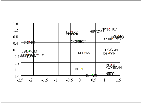
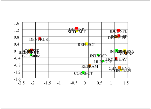
Dimensions 1 and 2 have been plotted in the next figure while dimensions
1 and 3 have been plotted in the subsequent figure.
The
figure gives a graphic picture of the distance between cluster 1 (from the
previous calculation; DEVTRUST, ACCEPT, BEINGNUR, and BGDMOM) and cluster 2
(SETLIMIT and DEFEXP). It also shows the
distance between cluster 1 and cluster 3 (DESENS and ADDRESA; the variable
CHALLENG is added to this cluster). Further, the distance between cluster 2 and
cluster 3 is presented in this graphic.
It is important to remember that the task as presented here is not to
test theory but develop taxonomies (in a sense to develop theory). The task is to help the researcher visualize
(understand) the complexities of the relationships among the variables.
Multidimensional
scaling provides information beyond cluster analysis as presented here. The two dimensions represented in the
circumplex provides to additional bits of information: (1) distance between the
clusters (and individual variables) and (2) where along each of dimensions each
variable and cluster lies. Although the
dendrogram in cluster analysis does provide information of the distance between
cluster 1 (INSIGHT, INTROSP, and INTERP) and cluster 3 (REFLECT and REFRAME) it
is a much clearer in the circumplex model of multidimensional scaling. Further, one can readily note the relation to
other clusters.
Multidimensional
scaling is not limited to two dimensions, like factor analysis there can be as
many dimensions as their are variables and in the same manner that there can be
as many factors as there are variables.
Unlike factor analysis the methods of determining the number of
dimensions is not as advanced as is the method for determining the number of
factors. As multidimensional scaling is
presented here that is not a problem
One could
think of these 21 elements being used to describe a school or style of
psychotherapy. In a simplified form
psychoanalysis might be thought of as made up of interpretation, transference
and countertransference, and working through.
This set
of statistics can be used on a range of taxonomic or descriptive problems. The creation of the input matrix determines
the issue studied. The method presented
here combined the data from a panel as described by Trochim. This process assists the clinician in sorting
out their judgments. However, a single
clinician could fill in the above chart by making judgments of the similarity
of the pairs (zero might represent similar--or no difference while 8 might represent
a great difference). In the cell
identified by ACCEPT (acceptance) and BEINGNUR (being nurturing) the judgment
might be 1 (quite similar). The cell
identified by DEVTRUST and CHALLENG might be judged 6 (quite dissimilar). The same set of statistics could then be
computed on the matrix of this single clinician. This would result in a map of the
clinician. Such maps could be used be
used in comparing theories. Students could
be compared to a panel of experts. These
methods could be used to empirically support the judgements of clinicians.
Personality
Theory Rating Scale
Name:
_________________________________________
Date: ________________
Use the scale below to rate the
personality theory of ____________________________.
╔═══════════════════════════════════════════════════════════════════════════╗
║
None A Little Somewhat Quite a Bit A Lot ║
╟───────────────────────────────────────────────────────────────────────────╢
║ 0 1
2 3 4
5 6 7
8 ║
╚═══════════════════════════════════════════════════════════════════════════╝
╔══════════════════════╗
║LEAVE
THE QUESTION ║
║BLANK IF
YOU DON'T ║
║KNOW OR
IF IT DOESN'T ║
║APPLY. ║
╚══════════════════════╝
ACCORDING
TO THIS THEORY:
_____
...motivation is based on drive reduction.
_____
...the person is an intentional (goal-oriented) being.
_____
...people are hedonistic.
_____
...cognition accounts for the actions of people.
_____
...values account for the actions of people.
_____
...people are actively involved in the development of their personality.
_____
...people's early experiences influence their personality.
_____
...the person imposes perception on the world.
_____
...the environment or learning accounts for the person's actions.
_____
...people are basically good.
_____
...heredity effects the person's actions.
_____
This theory stresses the individual's conscious view of the world.
_____
This theory stresses the individual's unconscious view of the world.
_____
This theory stresses the individual's social consciousness.
_____
This theory accounts for the individual's perception of reality.
_____
This theory has influenced psychology (clinical, research, literature).
_____
This theory focus on "the here and now", the past, or the
future.
(0 = past, 4 = here and now, 8 =
future)
_____
This theory is empirically based.
_____
This theory is parsimonious.
_____
This theory assumes that the individual has free choice.
_____
This theory employs a method of therapeutic intervention.
_____
This theory emphasizes psychopathology.
_____ I agree with this theory.
The names for the respective
items are as follows:
TDATE
THER
THID
CLUS
DRIVE
GOAL
HEDON
COG
VALUE
ACTIVE
EARLY
IMPOSE
LEARN
GOOD
HERED
CONSCI
UNCONS
SOCIAL
PERCEP
INFLU
TIME
DATA
PARSI
FREE
THERA
PATH
AGREE
The theorists rated were:
Freud Sigmund Freud
ADLER Alfred Adler
JUNG Carl Jung
ROGERS Carl Rogers
KELLY George Kelly
HORNEY Karen Horney
SULLIVI Harry Stack Sullivan
BANDURA Albert Bandura
CATTELL Raymond B. Cattell
MASLOW Abraham Maslow
BINSWAN Ludwig Binswanger
ERIKSON Erik Erikson
This data
was part of a graduate student class assignment for students taking a theories
of personality class. Each week the
students read the assignments and completed the questionnaire the day before
the class meeting. There were 17
students enrolled in the class, however, not all students complete the forms
each week and consequently there is some missing data. There were ___ completed forms.
In this
first example the items of the questionnaire are grouped using factor
analysis. Recall that in this condition
the items with similar profiles will be grouped together (into factors); not
necessarily the items that are closest in distance (refer to the above
discussion). The data is in a dBase IV
file with 9 indicating that data was omitted.
As can be seen mostly defaults were used in the computer run (see Frame
PERFAC5.SPS) and a principle components extraction method was used and the
rotation was orthoginal. Using the
eigenvalue of 1.00 is usually not considered the best method of deciding upon
the number of factors; however, both interpretation and the scree method seemed
also to indicate 5 factors.
|
File
Name = perfac5.sps
|
|
get file=
'\proeval\perall4.sav'/keep=
tDATE THER
THID CLUS DRIVE
GOAL HEDON COG
VALUE ACTIVE EARLY
IMPOSE LEARN
GOOD HERED CONSCI
UNCONS SOCIAL PERCEP
INFLU TIME
DATA PARSI FREE
THERA PATH AGREE .
missing values
drive to agree (9).
fac var= drive to
agree
/missing=pairwise
/plot=eigen
/criteria=factors(5)
/rotate.
|
┌────────────────────────────────────────────────────────────────────────────┐
│
PERFAC5.LIS
│
├────────────────────────────────────────────────────────────────────────────┤
│Final Statistics:
│
│
│
│Variable
Communality * Factor
Eigenvalue Pct of Var Cum Pct
│
│ *
│
│DRIVE
.54238 * 1
6.98937 30.4 30.4 │
│GOAL
.50485 * 2
2.15730 9.4 39.8 │
│HEDON
.54444 * 3
1.72904 7.5 47.3 │
│COG
.56063 * 4
1.47348 6.4 53.7 │
│VALUE
.66169 * 5
1.32890 5.8 59.5 │
│ACTIVE
.70979 *
│
│EARLY
.58670 *
│
│IMPOSE
.64661 *
│
│LEARN
.58716 *
│
│GOOD
.51995 *
│
│HERED
.58137 *
│
│CONSCI
.64024 * │
│UNCONS
.68112 *
│
│SOCIAL
.61566 *
│
│PERCEP
.61891 * │
│INFLU
.59501 *
│
│TIME
.58200 *
│
│DATA
.56921 *
│
│PARSI
.60125 *
│
│FREE
.61128 *
│
│THERA
.64608 *
│
│PATH
.52881 *
│
│AGREE
.54294 *
│
│
│
│Rotated Factor Matrix:
│
│
│
│
FACTOR 1 FACTOR
2 FACTOR 3
FACTOR 4 FACTOR
5 │
│
│
│DRIVE ‑.67035** ‑.10424 ‑.12588 ‑.21679 .13893
│
│GOAL
.44300 .44580* .16215 .17344 .23128
│
│HEDON ‑.72226** ‑.01600 .14498 .01324 .03653
│
│COG
.50422* .28914 .40228 .23887 ‑.06251 │
│VALUE
.15529 .79294** ‑.08091 ‑.04701 .00768
│
│ACTIVE
.58000** .41073 .21364
.39876 ‑.00630 │
│EARLY ‑.69231** .27344 ‑.13863 .07009 .09220
│
│IMPOSE
.22239 .23344 ‑.10607 .72878** .01706
│
│LEARN
.02767 .45879 .49137* .21355 ‑.29809 │
│GOOD
.57563** .41920 .00750 ‑.00350 .11316
│
│HERED
.10169 .28821 ‑.34325 ‑.60077** ‑.09606 │
│CONSCI
.55734** .40202 .29750 .26467 ‑.09712 │
│UNCONS ‑.48833* ‑.19803 ‑.48205 ‑.38498 .15119
│
│SOCIAL ‑.05895 .71266** .26140 .18852 .02080
│
│PERCEP
.29944 .16227 ‑.10921 .69839** .05684
│
│INFLU ‑.10405 .01029 .21463 ‑.17453 .71242**│
│TIME
.72841** .04942 .11085 .18045 ‑.06419 │
│DATA
.29151 .04499 .63344** ‑.20723 .19498
│
│PARSI
.05321 .06473 .76207** .00803 .11581
│
│FREE
.51295* .32588 .28510 .39853 .04315
│
│THERA ‑.13541 ‑.11914 ‑.26013 .24730 .69622**│
│PATH ‑.51195* ‑.08011 ‑.40072 ‑.11859 .29269
│
│AGREE ‑.01068 .34696 .25436 .21198 .55930**│
└────────────────────────────────────────────────────────────────────────────┘
We
were somewhat arbitrary in selecting 5 factors in this solution so that it
would match with the five cluster solution in the cluster analysis solution
that follows. It should be noted that
one should not be so casual in determining the number of factors in a solution;
the reader is referred to chapter __ when testing for the number of
factors. In developing theory the
researcher may do that in an armchair fashion, reviewing the literature or with
exploratory factor analysis. The major
purpose here to compare factor analysis with cluster analysis so that the
number of factors is done with that purpose in mind.
The
factors in Figure __ are presented in two ways: (1) the criterion of .60 is
used to determine whether a variable loads on a factor, (2) if a variable does
not load on any factor then it is placed on the factor with the highest
loading.
Factor I
DRIVE -.67
HEDON -.72
EARLY -.69
TIME .73
---------
GOAL .44
COG .50
ACTIVE .58
GOOD .58
CONSCI .56
UNCONS -.49
FREE .51
PATH -.51
Factor II
VALUE .79
SOCIAL .71
-----------
GOAL .45
Factor III
DATA .63
PARSI .76
----------
LEARN .49
Factor IV
IMPOSE .73
HERED -.60
PERCEP .70
Factor V
INFLU .71
THERA .70
AGREE .56
The next
example shows how cluster analysis can be used to group the same set of
data. The data needs to be conditioned
before the cluster analysis can be run.
The means are computed within each theorist for each item. For example, the first item DRIVE for all
respondents to Freud were summed and divided by the number of respondents (the
number was also rounded to the nearest integer to keep it on the same
scale). The matrix was then transposed
because the computer program requires that format for this problem. This data is presented in the frame THER11.sav.
|
ITEM
|
FREUD
|
ADLER
|
JUNG
|
ROGERS
|
KELLY
|
HORNEY
|
SULLIVA
|
BANDURA
|
CATTELL
|
MASLOW
|
BINSWAN
|
ERIKSON
|
|
DRIVE
|
8
|
2
|
3
|
2
|
2
|
3
|
4
|
1
|
3
|
4
|
2
|
4
|
|
GOAL
|
4
|
7
|
5
|
7
|
7
|
5
|
5
|
6
|
5
|
7
|
5
|
6
|
|
HEDON
|
7
|
3
|
2
|
2
|
2
|
4
|
4
|
2
|
3
|
4
|
3
|
3
|
|
COG
|
3
|
6
|
4
|
6
|
7
|
4
|
5
|
7
|
5
|
6
|
6
|
6
|
|
VALUE
|
4
|
6
|
5
|
6
|
4
|
4
|
5
|
5
|
4
|
6
|
6
|
6
|
|
ACTIVE
|
2
|
7
|
5
|
7
|
7
|
5
|
5
|
6
|
5
|
6
|
7
|
6
|
|
EARLY
|
8
|
7
|
4
|
5
|
4
|
6
|
6
|
5
|
4
|
5
|
4
|
7
|
|
IMPOSE
|
4
|
6
|
4
|
7
|
7
|
5
|
6
|
5
|
5
|
6
|
7
|
6
|
|
LEARN
|
3
|
6
|
3
|
5
|
5
|
6
|
6
|
7
|
6
|
5
|
5
|
6
|
|
GOOD
|
2
|
5
|
5
|
8
|
5
|
4
|
4
|
5
|
4
|
6
|
4
|
6
|
|
HERED
|
3
|
4
|
5
|
4
|
2
|
3
|
3
|
2
|
5
|
4
|
3
|
4
|
|
CONSCI
|
2
|
6
|
5
|
6
|
6
|
4
|
5
|
6
|
5
|
6
|
6
|
6
|
|
UNCONS
|
8
|
2
|
7
|
3
|
2
|
6
|
4
|
2
|
4
|
3
|
2
|
5
|
|
SOCIAL
|
4
|
7
|
3
|
6
|
5
|
5
|
6
|
6
|
5
|
5
|
5
|
6
|
|
PERCEP
|
5
|
6
|
5
|
7
|
7
|
5
|
6
|
6
|
5
|
6
|
7
|
5
|
|
INFLU
|
8
|
5
|
5
|
7
|
4
|
3
|
5
|
6
|
5
|
6
|
4
|
5
|
|
TIME
|
0
|
5
|
5
|
4
|
5
|
3
|
4
|
4
|
5
|
5
|
5
|
3
|
|
DATA
|
3
|
3
|
2
|
4
|
4
|
2
|
4
|
6
|
6
|
3
|
2
|
4
|
|
PARSI
|
4
|
5
|
3
|
5
|
6
|
4
|
4
|
5
|
5
|
5
|
3
|
5
|
|
FREE
|
2
|
5
|
3
|
7
|
7
|
5
|
4
|
6
|
4
|
6
|
7
|
5
|
|
THERA
|
7
|
5
|
6
|
7
|
6
|
5
|
6
|
5
|
3
|
3
|
5
|
5
|
|
PATH
|
7
|
3
|
5
|
3
|
3
|
6
|
5
|
3
|
4
|
3
|
4
|
4
|
|
AGREE
|
5
|
5
|
4
|
5
|
5
|
5
|
5
|
5
|
4
|
5
|
4
|
5
|
|
File
Name = percls3.sps
|
|
get
file = '\proeval\ther11.sav'/keep=
ITEM FREUD
ADLER JUNG ROGERS KELLY
HORNEY
SULLIVA BANDURA
CATTELL MASLOW BINSWAN
ERIKSON.
cluster
freud to erikson
/id=item
/print=distance
/print=schedule cluster(5)
/plot=dendrogram hicicle.
|
┌───────────────────────────────────────────────────────────────────────┐
│
PERCLS3.SPS
│
├───────────────────────────────────────────────────────────────────────┤
│Dendrogram using Average
Linkage (Between Groups)
│
│
│
│ Rescaled Distance
Cluster Combine │
│
│
│ C A S E 0
5 10 15 20 25
│
│ Label Seq
+‑‑‑‑‑‑‑‑‑+‑‑‑‑‑‑‑‑‑+‑‑‑‑‑‑‑‑‑+‑‑‑‑‑‑‑‑‑+‑‑‑‑‑‑‑‑‑+ │
│
│
│ IMPOSE 8
‑+‑+
│
│ PERCEP 15
‑+ |
│
│ GOAL 2
‑‑‑+‑+ │
│ COG 4
‑+ | | │
│ CONSCI 12
‑+‑+ +‑‑‑+ │
│ ACTIVE 6
‑+ | +‑+ │
│ FREE 20
‑‑‑‑‑+
| |
│
│ VALUE 5
‑‑‑‑‑‑‑+‑+ +‑‑‑‑‑‑‑‑‑+ │
│ GOOD 10
‑‑‑‑‑‑‑+ |
| │
│ LEARN 9
‑+‑‑‑‑‑+ |
| │
│ SOCIAL 14
‑+ +‑‑‑+ +‑‑‑‑‑‑‑‑‑‑‑+ │
│ PARSI 19
‑+‑‑‑‑‑+ | | │
│ AGREE 23
‑+ | | │
│ INFLU 16
‑‑‑‑‑‑‑‑‑‑‑‑‑+ | +‑‑‑‑‑‑‑‑‑‑‑‑‑‑‑+ │
│ THERA 21
‑‑‑‑‑‑‑‑‑‑‑‑‑+‑‑‑‑‑‑‑+ | | │
│ EARLY 7
‑‑‑‑‑‑‑‑‑‑‑‑‑+ | | │
│ HERED 11
‑‑‑‑‑‑‑‑‑‑‑‑‑‑‑+‑‑‑+ | | │
│ TIME 17
‑‑‑‑‑‑‑‑‑‑‑‑‑‑‑+ +‑‑‑‑‑‑‑‑‑‑‑‑‑+ | │
│ DATA 18
‑‑‑‑‑‑‑‑‑‑‑‑‑‑‑‑‑‑‑+ | │
│ DRIVE 1
‑+‑‑‑‑‑‑‑‑‑‑‑‑‑+ | │
│ HEDON 3
‑+ +‑‑‑‑‑‑‑‑‑‑‑‑‑‑‑‑‑‑‑‑‑‑‑‑‑‑‑‑‑‑‑‑‑+ │
│ UNCONS 13
‑‑‑‑‑+‑‑‑‑‑‑‑‑‑+ │
│ PATH 22
‑‑‑‑‑+ │
└───────────────────────────────────────────────────────────────────────┘
If five factors are chosen (to be
comparable to the 5 factor solution above) there are as follows:
Cluster
1
IMPOSE
PERCEP
GOAL
COG
CONSCI
ACTIVE
FREE
VALUE
GOOD
LEARN
SOCIAL
PARSI
AGREE
Cluster 2
INFLU
THERA
EARLY
Cluster 3
HERED
TIME
DATA
Cluster 4
DATA
Cluster 5
DRIVE
HEDON
UNCONS
PATH
The first
question is whether there is a difference between the factor analysis solution
and the cluster analysis solution? There
is not a test of significance that can be run [or would Chi Square be
appropriate? there is the problem of what is a match is it two or more
variables in the same group; cluseter or factor or must all overlap] so it is
mostly a matter determining whether it appears that the solutions are the same
or different. If one chooses to the
criteria of two or more variables in the same group then it does not look too
bad. Four variables from cluster 1 can
be found in factor 1; 3 variables from cluster 1 can be found in factor 2 (all
of factor 2); 2 variables in cluster 2 can be found in factor 5; and 4
variables in cluster 5 can be found in factor 1. That is 16 variables that overlap and 8
variables that do not [something wrong with this count]. That does give some indication that there is
some fit of the two methods. However,
cluster 3 does not have any variables that are shared in any of the factors and
factor 4 does not have any variables that are shared in any of the clusters. Further, cluster 1 and factor 1 are
fragmented across the two methods.
Finally, if one tries to develop a taxonomy from the two methods it
would seem to be different for the two methods.
|
File
Name = perals4.sps
|
|
get
file = '\proeval\therdtt.sav'/keep=
item
DRIVE GOAL
HEDON COG VALUE ACTIVE
EARLY
IMPOSE LEARN
GOOD HERED CONSCI
UNCONS SOCIAL
PERCEP INFLU
TIME DATA PARSI FREE
THERA
PATH AGREE.
ALS
VAR=drive to agree
/LEVEL=interval(disSIMILAR)
/PLOT=ALL.
|
┌─────────────────────────────────────────────────────────────────────┐
│ PERALS4.LST │
├─────────────────────────────────────────────────────────────────────┤
│ Configuration derived in 2
dimensions │
│ Stimulus Coordinates │
│ Dimension │
│Stimulus Stimulus
1 2 │
│
Number Name
│
│
│
│ 1
DRIVE 2.7576 ‑.0457 │
│ 2
GOAL ‑1.2316 .3747 │
│ 3
HEDON 2.2009 ‑.2654 │
│ 4
COG ‑1.2308 ‑.1352 │
│ 5 VALUE
‑.2718 .1322 │
│ 6
ACTIVE ‑1.7376 ‑.0292 │
│ 7
EARLY .2737 1.2230 │
│ 8
IMPOSE ‑1.1493 .3867 │
│ 9
LEARN ‑.8091 ‑.2012 │
│ 10
GOOD ‑.7062 ‑.5612 │
│ 11
HERED 1.1133 ‑.9480 │
│ 12
CONSCI ‑1.0615 ‑.3196 │
│ 13
UNCONS 2.4200 .6935 │
│ 14
SOCIAL ‑.5909 .1727 │
│ 15
PERCEP ‑1.0926 .6262 │
│ 16
INFLU .2361 .9594 │
│ 17
TIME ‑.2709 ‑1.4354 │
│ 18
DATA .7070 ‑1.3658 │
│ 19
PARSI .1220 ‑.2902 │
│ 20
FREE ‑1.3629 ‑.4720 │
│ 21
THERA .0554 1.0593 │
│ 22
PATH 1.4080 .3780 │
│ 23
AGREE .2212 .0633 │
└─────────────────────────────────────────────────────────────────────┘
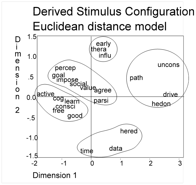
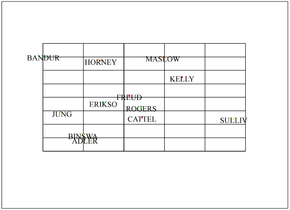
The Euclidean
Distance model in the above figure would seem to be helpful in developing a
taxonomy of the variables under consideration.
Outlines have been drawn to show the variables that might go together in
a group. The problem with the dispersion
is that there are no clear-cut distinctions between the variables; they seem to
be on a continuum. Consequently, the
divisions are somewhat arbitrary. It is
a little like dividing age ranges into ten year categories.
In keeping with the models above
of grouping the variables the following is the breakdown when five goups are
specified.
Group 1
EARLY
THERA
INFLU
Group 2
PERCEP
IMPOSE
GOAL
SOCIAL
VALUE
AGREE
PARSI
Group 3
UNCONS
PATH
DRIVE
HEDON
Group 4
ACTIVE
COG
LEARN
CONSI
FREE
GOOD
Group 5
HERED
TIME
DATA
In the
next example we use the same data set but focus on theorists rather than
variables. A taxonomy of theorists seems
as useful as a taxonomy of variables [must be a better way to say that]. Cattell's cube could be useful in this
context. The data used in the cluster
example is the same as the last cluster example but it was not transposed, it
is in Frame THER1.TXT.
|
FNAME
|
DRIVE
|
GOAL
|
HEDON
|
COG
|
VALUE
|
ACTIVE
|
EARLY
|
IMPOSE
|
LEARN
|
GOOD
|
HERED
|
CONSCI
|
UNCONS
|
SOCIAL
|
PERCEP
|
INFLU
|
TIME
|
DATA
|
PARSI
|
FREE
|
THERA
|
PATH
|
AGREE
|
|
FREUD
|
8
|
4
|
7
|
3
|
4
|
2
|
8
|
4
|
3
|
2
|
3
|
2
|
8
|
4
|
5
|
8
|
0
|
3
|
4
|
2
|
7
|
7
|
5
|
|
ADLER
|
2
|
7
|
3
|
6
|
6
|
7
|
7
|
6
|
6
|
5
|
4
|
6
|
2
|
7
|
6
|
5
|
5
|
3
|
5
|
5
|
5
|
3
|
5
|
|
JUNG
|
3
|
5
|
2
|
4
|
5
|
5
|
4
|
4
|
3
|
5
|
5
|
5
|
7
|
3
|
5
|
5
|
5
|
2
|
3
|
3
|
6
|
5
|
4
|
|
ROGERS
|
2
|
7
|
2
|
6
|
6
|
7
|
5
|
7
|
5
|
8
|
4
|
6
|
3
|
6
|
7
|
7
|
4
|
4
|
5
|
7
|
7
|
3
|
5
|
|
KELLY
|
2
|
7
|
2
|
7
|
4
|
7
|
4
|
7
|
5
|
5
|
2
|
6
|
2
|
5
|
7
|
4
|
5
|
4
|
6
|
7
|
6
|
3
|
5
|
|
HORNEY
|
3
|
5
|
4
|
4
|
4
|
5
|
6
|
5
|
6
|
4
|
3
|
4
|
6
|
5
|
5
|
3
|
3
|
2
|
4
|
5
|
5
|
6
|
5
|
|
SULLIVA
|
4
|
5
|
4
|
5
|
5
|
5
|
6
|
6
|
6
|
4
|
3
|
5
|
4
|
6
|
6
|
5
|
4
|
4
|
4
|
4
|
6
|
5
|
5
|
|
BANDURA
|
1
|
6
|
2
|
7
|
5
|
6
|
5
|
5
|
7
|
5
|
2
|
6
|
2
|
6
|
6
|
6
|
4
|
6
|
5
|
6
|
5
|
3
|
5
|
|
CATTELL
|
3
|
5
|
3
|
5
|
4
|
5
|
4
|
5
|
6
|
4
|
5
|
5
|
4
|
5
|
5
|
5
|
5
|
6
|
5
|
4
|
3
|
4
|
4
|
|
MASLOW
|
4
|
7
|
4
|
6
|
6
|
6
|
5
|
6
|
5
|
6
|
4
|
6
|
3
|
5
|
6
|
6
|
5
|
3
|
5
|
6
|
3
|
3
|
5
|
|
BINSWAN
|
2
|
5
|
3
|
6
|
6
|
7
|
4
|
7
|
5
|
4
|
3
|
6
|
2
|
5
|
7
|
4
|
5
|
2
|
3
|
7
|
5
|
4
|
4
|
|
ERIKSON
|
4
|
6
|
3
|
6
|
6
|
6
|
7
|
6
|
6
|
6
|
4
|
6
|
5
|
6
|
5
|
5
|
3
|
4
|
5
|
5
|
5
|
4
|
5
|
|
File Name = percls2.sps
|
|
get file = '\proeval\ther1.sav'/keep=
FNAME DRIVE GOAL HEDON
COG VALUE ACTIVE
EARLY
IMPOSE LEARN GOOD
HERED CONSCI UNCONS
SOCIAL PERCEP
INFLU TIME DATA
PARSI FREE THERA
PATH AGREE.
cluster drive to agree
/id=fname
/METHOD=WARD
/print=distance
/print=schedule
cluster(4)
/plot=dendrogram hicicle.
|
┌───────────────────────────────────────────────────────────────────────────┐
│
PERCLS2.LIS │
├───────────────────────────────────────────────────────────────────────────┤
│Cluster Membership of
Cases using Ward Method │
│
│
│ Number of
Clusters │
│ │
│ Label Case
4
│
│
│
│ Freud 1
1
│
│ Adler 2
2
│
│ Jung 3 3
│
│ Rogers 4
2
│
│ Kelly 5
2
│
│ Horney 6
4
│
│ Sulliva 7
4 │
│ Bandura 8
2
│
│ Cattell 9
4
│
│ Maslow 10
2 │
│ Binswan 11
2
│
│ Erikson 12
4
│
│
│
│Dendrogram using Ward
Method │
│
│
│ Rescaled Distance
Cluster Combine │
│ │
│ C A S E 0
5 10 15 20 25
│
│ Label Seq
+‑‑‑‑‑‑‑‑‑+‑‑‑‑‑‑‑‑‑+‑‑‑‑‑‑‑‑‑+‑‑‑‑‑‑‑‑‑+‑‑‑‑‑‑‑‑‑+ │
│ ┌─┐ ┌─┐ ┌─┐ │
│ │C│ │B│ │A│ │
│ Sulliva 7
‑+‑‑‑+ └┬┘ └┬┘ └┬┘ │
│ Erikson 12
‑+ +‑‑‑‑‑│‑+ │ │ │
│ Horney 6
‑‑‑‑‑+
│ +‑‑‑‑‑+ │ │ │
│ Cattell 9
‑‑‑‑‑‑‑‑‑‑‑│‑+ +‑‑‑│‑‑‑‑‑+ │ │
│ Jung 3
‑‑‑‑‑‑‑‑‑‑‑│‑‑‑‑‑‑‑+ │ |
│ │
│ Adler 2
‑+‑‑‑‑‑+ │ │ +‑‑‑‑‑‑‑‑│‑‑‑‑‑‑‑‑‑‑+ │
│ Maslow 10
‑+ +‑‑‑│‑‑‑+ │ |
│ |
│
│ Binswan 11
‑‑‑‑‑‑‑+ │ +‑‑‑‑‑‑‑│‑‑‑‑‑+ │ |
│
│ Kelly 5
‑‑‑+‑‑‑‑‑+ │ |
│ │ |
│
│ Bandura 8
‑‑‑+ +‑│‑‑‑+ │ │ |
│
│ Rogers 4
‑‑‑‑‑‑‑‑‑+ │ │ │ |
│
│ Freud 1
‑‑‑‑‑‑‑‑‑‑‑│‑‑‑‑‑‑‑‑‑‑‑│‑‑‑‑‑‑‑‑‑‑‑‑‑‑│‑‑‑‑‑‑‑‑‑‑+ │
└──────────────────────────────┴───────────┴──────────────┴─────────────────┘
Using the
rules of the vertical line should be
drawn at line "A" giving 2 clusters.
They are not very interesting in that Freud is in a cluster alone and
every other theorist is in the second cluster.
The next greatest horizontal distance is identified by line
"B" which forms two clusters.
This might be the might be interpretable set but line "C"
forming 6 clusters seems the most ______.
The clusters formed by this solution are as follows:
Cluster 1
Sullivan
Erikson
Horney
Cluster 2
Cattell
Cluster 3
Jung
Cluster 4
Adler
Maslow
Binswanger
Cluster 5
Kelly
Bandura
Rogers
Cluster 6
Freud
In this next set of data takes
same data as and
|
File Name = perals6.sps
|
|
get file = '\proeval\therdis1.sav'
/keep=
Freud Adler Jung
Rogers Kelly Horney
Sulliva Bandura Cattell
Maslow Binswan Erikson.
ALS VAR=Freud to Erikson
/LEVEL=interval(disSIMILAR)
/criteria=dimens(1)
/METHOD=INDSCAL
/PLOT=ALL.
|
┌──────────────────┐
│ PERALS6.LST │
├──────────────────┤
│KELLY ‑1.0647│
│ROGERS ‑0.9488│
│BANDURA ‑0.865 │
│BINSWAN ‑0.75
│
│ADLER ‑0.6355│
│MASLOW ‑0.3176│
│CATTELL 0.0888│
│ERIKSON 0.145 │
│SULLIVA 0.3638│
│HORNEY 0.591 │
│JUNG 0.7265│
│FREUD 2.6668│
└──────────────────┘
|
File Name = perals3.sps
|
|
get file = '\proeval\therdis1.sav'
/keep=
Freud Adler Jung
Rogers Kelly Horney
Sulliva Bandura Cattell
Maslow Binswan Erikson.
ALS VAR=Freud to Erikson
/LEVEL=interval(disSIMILAR)
/METHOD=INDSCAL
/PLOT=ALL.
|
|
File Name = therdis1.sav
|
|
FREUD
|
ADLER
|
JUNG
|
ROGERS
|
KELLY
|
HORNEY
|
SULLIVA
|
BANDURA
|
CATTELL
|
MASLOW
|
BINSWAN
|
ERIKSON
|
|
0
|
249
|
145
|
276
|
295
|
121
|
126
|
270
|
189
|
218
|
263
|
167
|
|
249
|
0
|
96
|
33
|
34
|
66
|
33
|
29
|
52
|
23
|
34
|
24
|
|
145
|
96
|
0
|
103
|
110
|
46
|
55
|
115
|
58
|
77
|
82
|
66
|
|
276
|
33
|
103
|
0
|
33
|
101
|
60
|
38
|
81
|
36
|
49
|
39
|
|
295
|
34
|
110
|
33
|
0
|
84
|
55
|
27
|
64
|
39
|
28
|
54
|
|
121
|
66
|
46
|
101
|
84
|
0
|
23
|
83
|
50
|
65
|
62
|
38
|
|
126
|
33
|
55
|
60
|
55
|
23
|
0
|
44
|
31
|
38
|
43
|
19
|
|
270
|
29
|
115
|
38
|
27
|
83
|
44
|
0
|
43
|
42
|
47
|
41
|
|
189
|
52
|
58
|
81
|
64
|
50
|
31
|
43
|
0
|
39
|
62
|
40
|
|
218
|
23
|
77
|
36
|
39
|
65
|
38
|
42
|
39
|
0
|
35
|
25
|
|
263
|
34
|
82
|
49
|
28
|
62
|
43
|
47
|
62
|
35
|
0
|
54
|
|
167
|
24
|
66
|
39
|
54
|
38
|
19
|
41
|
40
|
25
|
54
|
0
|
┌──────────────────────────────────────────────────┐
│ PERALS3.LST │
├──────────────────────────────────────────────────┤
│ Dimension 1 Dimension 2 │
│
│
│KELLY ‑1.4323 JUNG ‑0.9577 │
│ROGERS ‑1.2329 CATTELL ‑0.7267 │
│BANDURA ‑1.1546 BINSWAN ‑0.653 │
│BINSWAN ‑0.9693 KELLY ‑0.2254 │
│ADLER ‑0.8148 HORNEY ‑0.0529 │
│MASLOW ‑0.3965 FREUD 0.1277 │
│CATTELL 0.0739 SULLIVA 0.1736
│
│ERIKSON 0.2 BANDURA 0.3124
│
│SULLIVA 0.51 ERIKSON 0.4641
│
│JUNG 0.8239 ADLER 0.4963 │
│HORNEY 0.84 ROGERS 0.5 │
│FREUD 3.545 MASLOW 0.5358 │
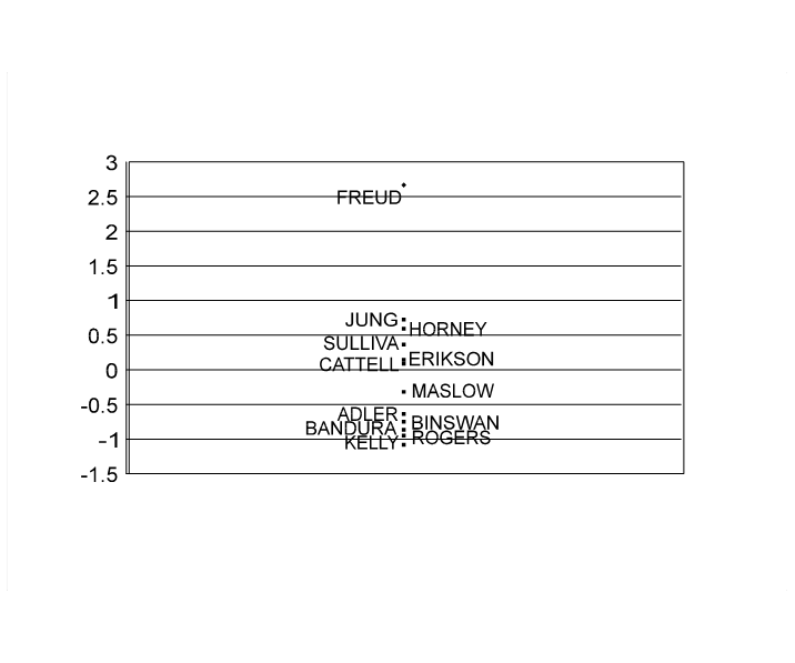
└──────────────────────────────────────────────────┘
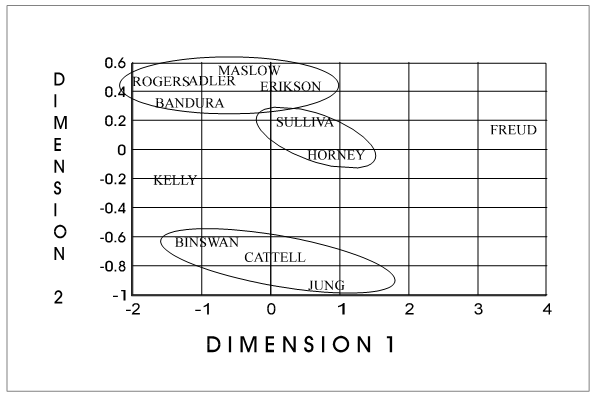
It
produced the following chart:
Cluster
analysis and multidimensional are the similar when multidimensional scaling
uses only one dimension. This can be
seen in comparing Dimension 1 and the Dendogram (not real sure of this one at
this point--I'll check it further).
The
manner in which the data is entered for these programs makes a major difference
in the results. It is as important as
choosing the proper statistics. In the
above example there were ______ manipulations of the data before it was entered
into the program. The participants
completed a questionnaire about the theorists, each item was summed across the
participants within each theorist, and the squared multiple distance between
each theorist was computed. It was the
squared multiple distance that was used as input to the multidimensional
scaling program. In the following
example the input to the program are direct judgments of a single judge. The judge makes a decision about the distance
between each pair of objects (in this instance personality theorists) based on
personal attitudes, information, or __________.
A single
judge compared each theorist by using a scale from 0 to 8. A zero (0) indicated that the theorists were
identical and an 8 indicated that the theorists were most dissimilar. The judge rated Freud and Adler as similar
with a 3, and rated Jung as slightly more similar to Freud with a 2. The rating of Bandura to Freud with an 8
indicates most dissimilarity.
|
File
Name = therate.sav
|
|
THEORIST
|
FREUD
|
ADLER
|
JUNG
|
ROGERS
|
KELLY
|
HORNEY
|
SULLIVA
|
BANDURA
|
CATTELL
|
MASLOW
|
BINSWAN
|
ERIKSON
|
|
FREUD
|
0
|
3
|
2
|
5
|
6
|
4
|
4
|
8
|
8
|
5
|
6
|
5
|
|
ADLER
|
3
|
0
|
3
|
4
|
3
|
4
|
2
|
5
|
4
|
3
|
3
|
4
|
|
JUNG
|
2
|
3
|
0
|
4
|
3
|
4
|
3
|
7
|
7
|
2
|
2
|
4
|
|
ROGERS
|
5
|
4
|
4
|
0
|
3
|
5
|
3
|
5
|
6
|
2
|
3
|
5
|
|
KELLY
|
6
|
3
|
3
|
3
|
0
|
2
|
2
|
2
|
3
|
3
|
5
|
3
|
|
HORNEY
|
4
|
4
|
4
|
5
|
2
|
0
|
2
|
4
|
3
|
4
|
4
|
2
|
|
SULLIVA
|
4
|
2
|
3
|
3
|
2
|
2
|
0
|
3
|
2
|
3
|
4
|
1
|
|
BANDURA
|
8
|
5
|
7
|
5
|
2
|
4
|
3
|
0
|
2
|
4
|
4
|
3
|
|
CATTELL
|
8
|
4
|
7
|
6
|
3
|
3
|
2
|
2
|
0
|
3
|
3
|
2
|
|
MASLOW
|
5
|
3
|
2
|
2
|
3
|
4
|
3
|
4
|
3
|
0
|
1
|
4
|
|
BINSWAN
|
6
|
3
|
2
|
3
|
5
|
4
|
4
|
4
|
3
|
1
|
0
|
3
|
|
ERIKSON
|
5
|
4
|
4
|
5
|
3
|
2
|
1
|
3
|
2
|
4
|
3
|
0
|
The
jobstream used to run the multidimensional scaling program in SPSS is as
follows:
|
File Name = perals9.sps
|
|
get file = '\proeval\therate.sav'
/keep=
THEORIST FREUD ADLER
JUNG ROGERS
KELLY HORNEY SULLIVA
BANDURA CATTELL MASLOW
BINSWAN ERIKSON.
ALS VAR=FREUD TO ERIKSON
/LEVEL=INTERVAL(disSIMILAR)
/PLOT=ALL.
|
It should
be noted that the text file "THERATE.TXT" did not contain the names
of the theorists on the first line. The
output of that computer run is in Frame PERALS9.LST. One might ask the whether the two matrices
are different. For example, the group of
judges might have been a panel of experts and the single rater might be a
student and the question would be how close to the experts is the student? On the other hand the categories might be
diagnosis and the question might be different methods of establishing
diagnoses: (1) structured interview, (2) psychological testing, or (3) clinical
judgment. There could seem to be a whole
set of clinical judgment questions that these methods could be applied to.
We
indicated in the above section that there is not a statistical method for
determining the grouping solutions of
cluster analysis, factor analysis, or multidimensional scaling was different
among themselves. However, there are
methods for determining whether the matrices themselves are significantly
different.
┌────────────────────────────┐
│ PERALS9.LST │
├────────────────────────────┤
│ Dimension │
│ │
│Stimulus 1
2 │
│ Name │
│ │
│Freud 2.1751
.8550 │
│ADLER .8344
.3116 │
│JUNG 1.5860
‑.1741 │
│ROGERS .6082
‑1.5110 │
│KELLY ‑.6659 .3442
│
│HORNEY ‑.2005 1.1608
│
│SULLIVA ‑.1193 .4693
│
│BANDURA ‑1.8848 ‑.1841
│
│CATTELL ‑1.7805 .1339
│
│MASLOW .1183
‑.9897 │
│BINSWAN ‑.0561 ‑1.2390
│
│ERIKSON ‑.6148 .8230
│
└────────────────────────────┘
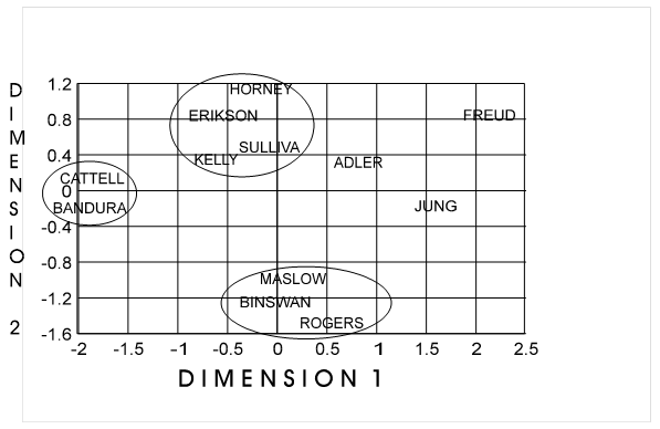
That
data from Frame PERALS9.LST was used to create the following plot:
If the
categories are known then it might be desirable to predict the theorist. Discriminant analysis allows one to determine
which variables are most effective in predicting theorists and to develop a
taxonomy for both the theorist and the variables.
|
File Name = perdsc2.sps
|
|
get file = '\proeval\perall4.sav'/keep=
THID
CLUS DRIVE
GOAL
HEDON COG VALUE ACTIVE
EARLY IMPOSE LEARN
GOOD
HERED CONSCI UNCONS
SOCIAL PERCEP INFLU
TIME
DATA
PARSI FREE THERA PATH
AGREE .
value labels thid
1
'freud'
2
'Adler'
3
'Jung'
4
'Rogers'
5
'Kelly'
6
'Horney'
7
'Sulliva'
8
'Bandura'
9
'Cattell'
10
'Maslow'
11
'Binswan'
12
'Erikson'.
missing values drive to agree (9).
DSC GROUPS=thid(1,12)
/VAR=drive to agree
/METHOD=MINRESID
/PIN=.05
/FUNCTIONS=6,100,.05
/STATISTICS=MEAN STDDEV COEFF RAW TABLE.
|
Degrees of
Freedom Signif. Between Groups
Wilks' Lambda .00238 18
11 172.0
Approximate F 6.73348 198 1487.7
.0000
RESIDUAL VARIANCE 12.98197
‑‑‑‑‑‑‑‑‑‑‑‑‑‑‑‑
Variables in the analysis after step 18 ‑‑‑‑‑‑‑‑‑‑‑‑‑‑‑‑
Variable
Tolerance F to remove Residual Variance
DRIVE
.8086075 4.4085
GOAL
.6885392 2.8517
HEDON
.8205188 4.2216
VALUE
.6899227 1.8635
EARLY
.7400657 4.8709
LEARN
.7701072 2.5441
GOOD
.7114397 8.9138
HERED
.8461894 3.0091
CONSCI
.5652705 3.7762
UNCONS
.5666565 4.9305
SOCIAL
.6762921 2.1756
PERCEP
.8453969 3.0534
INFLU
.7347672 9.9031
DATA .7400053
7.9982
FREE
.7024298 3.1230
THERA
.6631685 4.7735
PATH
.6396031 4.2841
AGREE
.7558803 2.3188
‑‑‑‑‑‑‑‑‑‑‑‑‑‑‑‑
Variables not in the analysis after step
18 ‑‑‑‑‑‑‑‑‑‑‑‑‑‑‑‑
Minimum Signif. of
Variable
Tolerance Tolerance F to enter
Residual variance
COG
.7229042 .5566498 .6106
ACTIVE
.5912503 .5277644 .2419
IMPOSE
.6659893 .5559298 .6726
TIME
.7545682 .5623679
.0731
PARSI
.7565332 .5601723 .2784
Canonical Discriminant Functions evaluated at
Group Means (Group Centroids)
Group
FUNC 1 FUNC
2 FUNC 3
FUNC 4 FUNC
5
1
5.95297 .15154 .28629 .05561
‑1.15760
2
‑.63536 ‑.27522 ‑.00035 1.83737
‑.15173
3
1.02702 1.23000 .55006
‑1.87012 .81240
4
‑1.46471 1.63556 1.68544 .26381
‑.08564
5
‑2.42486 .46351 ‑.56310 ‑.62008 ‑1.47778
6
.87926 ‑.12746 ‑2.36745 .13268
1.08705
7
.37195 ‑.86906 ‑.85952 .27647 .40472
8
‑1.46161 ‑1.49840 .54719
.30448 ‑.86419
9
‑.59271 ‑2.65032 1.03258
‑1.18762 .46617
10
‑.35662 .98185 .87905 .46556 .93586
11
‑1.59251 .96399 ‑1.73615 ‑.52494 ‑.44835
12
.31087 ‑.05714 .48770 .58778
1.10934
Group
FUNC 6
1
‑.26492
2
.35772
3
.83661
4
.56233
5
.58221
6
.63629
7
.35528
8
.01865
9
‑.44479
10
‑1.26531
11
‑1.41790
12
.27400
Pooled‑within‑groups correlations
between discriminating variables
and
canonical discriminant functions
(Variables ordered by size of correlation
within function)
FUNC 1
FUNC 2 FUNC
3 FUNC 4
FUNC 5 FUNC
6
UNCONS
.48407* .03096 ‑.09763 ‑.35571* .26928
.43638*
DRIVE
.45355* .01335
.05730 ‑.03132 .06143
‑.3268*
CONSCI
‑.44664* .02689 .14508
.15771 .00853 ‑.08340
ACTIVE
‑.41748* .02171 .18051
.18981 ‑.10032 ‑.03243
FREE
‑.37396* .27632 .00144
.13380 ‑.16393 ‑.28372
HEDON
.33958* ‑.05369 ‑.10844 .32823*
.00075 ‑.17824
PATH
.32608* ‑.00935 ‑.31459* ‑.10368 .08268
.15747
TIME
‑.31732* .14655 .07322
‑.02276 ‑.11320 .03428
COG
‑.28334* ‑.01902 .17173
.14983 ‑.06110 ‑.12010
DATA
‑.15986 ‑.46128* .36008
‑.07347 ‑.14761 .06128
LEARN
‑.25227 ‑.38030* ‑.03127 .34017*
.16834 .15273
PARSI
‑.03410 ‑.12764 .09310
‑.00652 ‑.04193 ‑.04799
INFLU
.22419 .10896 .57515*
.13349 ‑.29370 ‑.05110
EARLY
.26233 ‑.04628 ‑.10997 .51862*
.03825 .27307
SOCIAL
‑.12369 ‑.12257 .03867
.49163* .13589 .01540
GOAL
‑.20539 .14144 .25223
.30214* ‑.06513 .00034
VALUE
‑.09861 .13987 .12987
.29536 .28964 ‑.26646
AGREE
‑.01220 .18610 .06580
.25217 ‑.14317 .12416
GOOD
‑.33015* .36429* .32580*
.29638 .44471* .18545
HERED
.04960 ‑.11310 .24118
‑.18815 .36794* ‑.06445
PERCEP
‑.23170 .20847 .00742
.19155 ‑.28685* ‑.03778
IMPOSE
‑.14642 .12907 .00069
.13448 ‑.17966* .01658
THERA
.12568 .27235 .02229
.00194 ‑.45201* .50039*
No. of Predicted Group Membership
Actual
1 2 3
4 5 6
7 8 9
10 11 12
Freud
100.0 .0 .0
.0 .0 .0
.0 .0 .0
.0 .0 .0
Adler
.0 58.8 .0
11.8 .0 .0
11.8 11.8 .0
.0 .0 5.9
Jung
.0 .0 100.0 .0
.0 .0 .0 .0
.0 .0 .0
.0
Rogers
.0 .0 .0
81.3 .0 .0
.0 .0 .0
12.5 .0 6.3
Kelly
.0 11.8 .0
5.9 76.5 .0
.0 .0 .0
.0 5.9 .0
Horney
.0 .0 6.7
.0 6.7 73.3
6.7 .0 .0
.0 6.7 .0
Sulliva
.0 18.8 12.5
.0 .0 18.8
37.5 .0 .0
.0 6.3 6.3
Bandura
.0 6.3 .0
.0 12.5 .0
6.3 75.0 .0
.0 .0 .0
Cattell
.0 .0 6.7
.0 .0 .0
.0 6.7 86.7
.0 .0 .0
Maslow
.0 11.8 5.9
.0 .0 .0
.0 .0 .0
76.5 5.9 .0
Binswan
.0 .0 .0
.0 .0 .0
.0 .0 .0
6.7 93.3 .0
Erikson
.0 8.3 8.3
8.3 .0 .0
8.3 .0 .0
.0 .0 66.7
Percent of "grouped"
cases correctly classified: 77.25%
The Y-hat
formula that was generated by these show that level of prediction of each of
the categories or in this case the theorists.
That is, by knowing how the a theorist is rated on each of the items it
can be predicted which theorists it is.
The level that each theorist is predicted is known.
Two sets
of data from the output are useful in interpreting this data: (1)
"Structure Matrix", and (2) the "Canonical Discriminant
Functions evaluated and Group Means (Group Centroids)." Plotting these two sets of data presents a
pictures of the taxonomy of characteristics of variables and theorists. It is necessary to first define the Structure
Matrix and the Functions/Centroids.
The
discriminant function is a prediction equation much like a in multiple
regression. The definition in chapter __
defines this general linear model. In
discriminant as set of predictor variables predicts a set of groups. The first discriminant function seperates the
groups most effectively and if the variables contain variance (information)
such that the groups can be more accurately seperated a second discriminant
function is computed and so on until there is no more variance among the groups
that can be seperated by the variables.
The discriminant functions can be described by the variables that load
on them in much the same manner as factor analysis.
The
discriminant function can be used to make a prediction for each case. When these cases are summed within each group
and divided by the number of cases in that group these means are called
centroids. The greater difference among
the means is the goal of discriminant function.
These means can be plotted to identify which functions are seperating
which groups. Further, when the
functions are defined by the variable loadings then a taxonomy of the variables
can be related to the groups. In the
case we are dealing with this means that the characteristics of a theory can be
empirically related to the theory.
We
arbitrarly requested 6 functions in the program (realizing that 9 function are
significant) to demonstrate how the discriminant function can be
interpreted. Further we plot the group
centroids to show their discriminating power for the various theorists. We used only 3 2-way plots even though there
is a possiblility of 15. It does show
the discriminating power of all 6 functions for all 12 theorists; it just does
not show all combinations. For example,
it shows function 1 with function 2 but does not show function 1 with 3, 4, 5,
or 6. Although these might be
interesting space does not allow presentation of all combinations. The three presented should be useful in the
interpretation .... In fact, it might
have been as useful to show the discriminating power for each of the functions
independently.
The
functions are also like the dimensions in multidimensional scaling, but are
different in that there is a criterion variable in the discriminate
function. Further, the discriminant
function allows ... The graphs are
created by using (1) "Structure Matrix", and (2) the "Canonical
Discriminant Functions evaluated and Group Means (Group Centroids)" as
mentioned above. First the plots are
created by using the data from the Group Centroids. For example, notice in the first figure that
Freud is to the far right with a score of 5.95 on Function 1. Jung, Horney, Erikson, and Sullivan are near
the center with scores of 1.03, .88, .31 and .37 respectively. On Function 2 Rogers has the most positive
score of 1.64 while Cattell has the most negative score of -2.65. These functions are defined by the variables
that correlate with them. Function 1 is
made up of Uncons, Consci, Drive, Active, Free, Hedon, Path, and Time. Function 2 is made up of Data, Learn, and
Good.
These
functions can be interpreted like factors of factor analsysis. The first function might be labeled
"unconscious motivation" at one pole and conscious decision making at
the other. It is this that seperates
Freud from most other theorists. Kelly,
Bandura, and Cattell are at the conscious decision making end of the continuum. Function 2 is made up of Data, Learn, and
Good. Good is in the positive direction
and Data and Learning are at the negative end of the function. So that Rogers sees individuals as good, his
theory is not based on empirical evidence and learning does not account for
much of peoples' actions. On the other
hand, the theories of Cattell and Bandura data and learning have considerable
impact on individuals but they are not seen as intrinsically good (one cannot
conclude that they assume people are intrinsically bad).
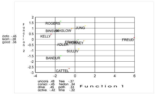
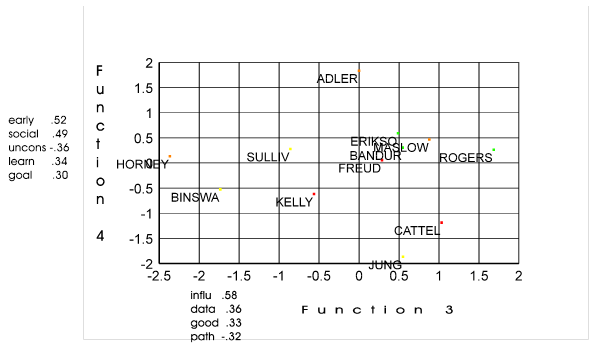
In Figure
__ Function 3 is not as clear Influ (influence), Data, Good, and Path
(negative) do not seem to hang together very well. However, they are the variables that seperate
Horney and Binswanger from Rogers, Maslow and Cattell.
Seventy-seven
percent correctly classified is decent prediction so that one would conclude
that the instrument is reliable is distinguishing among different personality
theories. However, the instrument was
not very effective in predicting Adler (58%) and Sullivan (37%), further
Erikson with 67% could also be improved.
In diagnosing the problem it can be seen that the misses for Adler were
with Rogers (12% misses for Adler were predicted to be Rogers), Sullivan, and
Bandura (each with 12%). One might hypothesize
that the theory of Adler is similar to that of Rogers, Sullivan, and Bandura
and it is not the problem with the measuring device. Further, it might be hypothesized that
Sullivan is similar to Adler, Jung, and Horney (19%, 13%, and 19% respectively). This notion could be tested by combining the
theories such that similar theorist would be in the same categories. Another analysis was run with Adler and
Sullivan combined into
a single category and the overall
percentage of correct predictions went up slight to 79%. The Adler Sullivan category was 54% correctly
predicted, still somewhat low. Further,
this did not correct some of the overlap indicated. It would be more advantages to see if there
might be a way to separate the theorists.
The
output from the first run indicates that there are more than 6 functions that
are significant. In fact there are 9
functions that are significant. A
jobstream was run requesting 9 functions and the percent correctly predicted
rose to 85%.
|
File Name = perdsc9.sps
|
|
get
file = '\proeval\perall4.sav'/keep=
THID CLUS DRIVE
GOAL HEDON COG
VALUE ACTIVE EARLY
IMPOSE LEARN
GOOD HERED CONSCI
UNCONS SOCIAL PERCEP
INFLU TIME
DATA PARSI
FREE THERA PATH
AGREE .
value
labels thid
1 'freud'
2 'Adler'
3 'Jung'
4 'Rogers'
5 'Kelly'
6 'Horney'
7 'Sulliva'
8 'Bandura'
9 'Cattell'
10 'Maslow'
11 'Binswan'
12 'Erikson'.
missing
values drive to agree (9).
DSC
GROUPS=thid(1,12)
/VAR=drive to agree
/METHOD=MINRESID
/PIN=.05
/FUNCTIONS=6,100,.05
/STATISTICS=MEAN STDDEV COEFF RAW TABLE.
|
Canonical Discriminant
Functions
Pct of Cum
Canonical After Wilks'
Fcn Eigenvalue Variance Pct
Corr Fcn Lambda
Chisquare DF Sig
: 0
.0024 1014.589 198
.0000
1*
4.9499 45.38 45.38
.9121 : 1 .0142
714.982 170 .0000
2*
1.4590 13.38 58.76
.7703 : 2 .0349
563.823 144 .0000
3*
1.3565 12.44 71.19
.7587 : 3 .0822
419.820 120 .0000
4*
.8325 7.63 78.82
.6740 : 4 .1506
318.062 98 .0000
5*
.7967 7.30 86.13
.6659 : 5 .2706
219.621 78 .0000
6*
.5371 4.92 91.05 .5911 :
6 .4159 147.401
60 .0000
7*
.2945 2.70 93.75
.4770 : 7 .5383
104.040 44 .0000
8*
.2782 2.55 96.30
.4666 : 8 .6881
62.799 30 .0004
9*
.1903 1.75 98.05
.3999 : 9 .8191
33.525 18 .0144
10
.1662 1.52 99.57
.3775 : 10 .9552
7.693 8 .4640
11
.0469 .43 100.00
.2116 :
Structure
Matrix:
Pooled‑within‑groups
correlations between discriminating variables
and canonical
discriminant functions
(Variables
ordered by size of correlation within function)
FUNC 1
FUNC 2 FUNC
3 FUNC 4
FUNC 5 FUNC
6
UNCONS .48407* .03096
‑.09763 ‑.35571* .26928
.43638*
CONSCI ‑.44664* .02689
.14508 .15771 .00853
‑.08340
ACTIVE ‑.41748* .02171
.18051 .18981 ‑.10032 ‑.03243
FREE ‑.37396* .27632
.00144 .13380 ‑.16393 ‑.28372
HEDON .33958* ‑.05369 ‑.10844 .32823*
.00075 ‑.17824
TIME ‑.31732* .14655
.07322 ‑.02276 ‑.11320 .03428
COG ‑.28334* ‑.01902 .17173
.14983 ‑.06110 ‑.12010
DATA ‑.15986 ‑.46128* .36008*
‑.07347 ‑.14761 .06128
LEARN ‑.25227 ‑.38030* ‑.03127 .34017*
.16834 .15273
INFLU .22419 .10896
.57515* .13349 ‑.29370 ‑.05110
EARLY .26233 ‑.04628 ‑.10997 .51862*
.03825 .27307
SOCIAL ‑.12369 ‑.12257 .03867
.49163* .13589 .01540
VALUE ‑.09861 .13987
.12987 .29536* .28964
‑.26646
AGREE ‑.01220 .18610
.06580 .25217* ‑.14317 .12416
GOOD ‑.33015* .36429*
.32580* .29638* .44471*
.18545
THERA .12568 .27235
.02229 .00194 ‑.45201* .50039*
GOAL ‑.20539 .14144
.25223 .30214* ‑.06513 .00034
DRIVE .45355* .01335
.05730 ‑.03132 .06143
‑.32682*
PERCEP ‑.23170 .20847
.00742 .19155 ‑.28685 ‑.03778
IMPOSE ‑.14642 .12907
.00069 .13448 ‑.17966 .01658
HERED .04960 ‑.11310 .24118
‑.18815 .36794* ‑.06445
PATH .32608* ‑.00935 ‑.31459* ‑.10368 .08268
.15747
PARSI ‑.03410 ‑.12764 .09310
‑.00652 ‑.04193 ‑.04799
FUNC 7
FUNC 8 FUNC
9
UNCONS ‑.18115 ‑.00945 .01236
CONSCI .09633 ‑.10474 ‑.17831
ACTIVE ‑.02584 ‑.06411 .09399
FREE .04931 ‑.09084 .30007*
HEDON .10374 .22748
.11044
TIME .08627 .02253
.03357
COG ‑.01675 ‑.03132 .09982
DATA .14982 .12043
.24718
LEARN .26302 .08228
.29436
INFLU .28069 ‑.17830 .17723
EARLY ‑.06572 ‑.14613 ‑.15911
SOCIAL .30753* ‑.00789 ‑.23385
VALUE .27222 ‑.24204 ‑.08582
AGREE ‑.06715 ‑.04745 .24494
GOOD .17276 .04759
.14258
THERA .40108* .05956
‑.35879
GOAL ‑.33333* .09962
‑.09469
DRIVE .05246 .54241*
‑.08198
PERCEP ‑.02293 .47956*
‑.08374
IMPOSE ‑.08930 .19274*
‑.12481
HERED ‑.28983 ‑.07839 ‑.45725*
PATH .27487 .15742
‑.43764*
PARSI .09651 ‑.03737 .25767*
Canonical
Discriminant Functions evaluated at Group Means (Group Centroids)
Group
FUNC 1 FUNC
2 FUNC 3
FUNC 4 FUNC
5
1
5.95297 .15154 .28629 .05561
‑1.15760
2
‑.63536 ‑.27522 ‑.00035 1.83737
‑.15173
3
1.02702 1.23000 .55006
‑1.87012 .81240
4
‑1.46471 1.63556 1.68544 .26381
‑.08564
5
‑2.42486 .46351 ‑.56310 ‑.62008 ‑1.47778
6
.87926 ‑.12746 ‑2.36745 .13268
1.08705
7
.37195 ‑.86906 ‑.85952 .27647 .40472
8
‑1.46161 ‑1.49840 .54719 .30448
‑.86419
9
‑.59271 ‑2.65032 1.03258
‑1.18762 .46617
10
‑.35662 .98185 .87905
.46556 .93586
11
‑1.59251 .96399 ‑1.73615 ‑.52494 ‑.44835
12
.31087 ‑.05714 .48770 .58778
1.10934
Group
FUNC 6 FUNC
7 FUNC 8
FUNC 9
1
‑.26492 ‑.06609 .05194 .02423
2
.35772 ‑.65579 ‑.38601 ‑.62244
3
.83661 .03531 ‑.61179 ‑.22382
4
.56233 .49353 .17086
‑.14415
5
.58221 ‑.69567 .57408 .29868
6
.63629 ‑.19940 ‑.22853 .54813
7
.35528 .97323 1.08427
‑.31534
8
.01865 .78145 ‑.79608 .61210
9
‑.44479 ‑.50719 .17872
‑.29761
10
‑1.26531 ‑.27827 .38276 .59534
11
‑1.41790 .32617 ‑.40514 ‑.55439
12
.27400 ‑.13150 ‑.20468 ‑.07838
Classification
Results ‑
No. of Predicted Group Membership
Actual 1
2 3 4
5 6 7
8 9 10
11 12
Freud 100.0 .0
.0 .0 .0
.0 .0 .0
.0 .0 .0
.0
Adler .0 70.6
.0 5.9 5.9
.0 .0 .0
.0 5.9 .0
11.8
Jung .0 .0
93.8 .0 .0
.0 .0 .0
.0 .0 .0
6.3
Rogers .0 .0
.0 100.0 .0 .0
.0 .0 .0
.0 .0 .0
Kelly .0 5.9
.0 11.8 76.5
.0 .0 5.9
.0 .0 .0
.0
Horney .0 .0
.0 .0 6.7
86.7 6.7 .0
.0 .0 .0
.0
Sulliva .0 .0
12.5 .0 .0
18.8 56.3 .0
.0 .0 .0
12.5
Bandura .0 .0
.0 .0 6.3
.0 .0 93.8
.0 .0 .0
.0
Cattell .0 .0
.0 .0 .0
.0 6.7 .0
93.3 .0 .0
.0
Maslow .0 5.9
5.9 5.9 .0
.0 .0 .0
.0 70.6 11.8
.0
Binswan .0 .0
.0 .0 .0
.0 .0 .0
.0 .0 100.0 .0
Erikson .0 8.3
.0 8.3 .0
.0 .0 .0
.0 .0 .0
83.3
Eighty-Five
of the cases were correctly classified.
This represents an improvement over the previous run where 77% of cases
were correctly classified. It was noted
above the that the 6 function solution did not discriminate well on the
theorists Adler, Jung, Rogers, Horney, Sullivan, Bandura, and Erikson. Figures __ and __ demonstrate that Functions
7, 8, and 9 performed that task. Figure __
shows Functions 7 and 8; on Function 7 Sullivan and Bandura are on one
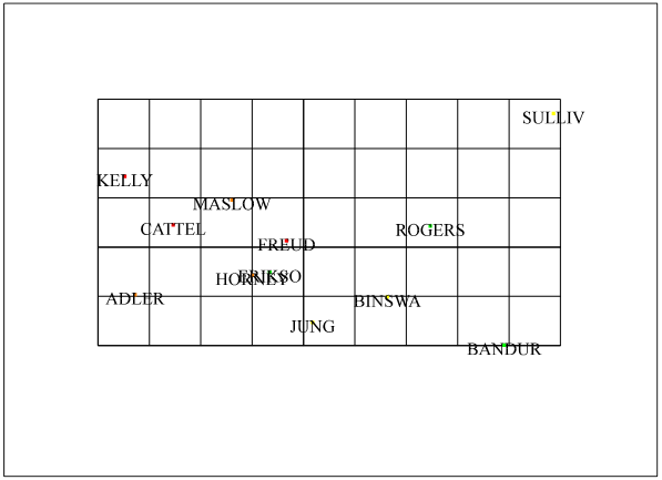
end of the continuum and Kelly
and Adler at the other end of the continuum.
Further, Erikson and Horney are to the left while Rogers is to the
right. Function 8 seperates Sullivan and
Kelly from Erikson, Horney, Adler, Jung and Bandura. And finally Function 9 seperates Adler and
Sullivan from Bandura and Horney.