Chapter 11
Factor Analysis
Merle Canfield, Ph.D.
Factor analysis takes a set of correlations
and finds a solution such that variables that are correlated together form a
factor that is not related to other factors.
It summarizes the correlation matrix.
It can be thought of as reducing the redundancy in a set of
correlations. It is assumed that there
is an underlying factor or variable that results in the variables being
related. From a theoretical point of
view this is the epitome of taking advantage of chance correlations. The variables are the manifestations of the
underlying factor or variable.
There five general uses of factor analysis
as presented here: (1) summarizing data of a correlation matrix, (2) reducing
data, (3) constructing tests, (3) building theory (identifying underlying
factors), (4) generating Y' for each factor, and (5) selecting a smaller set of
variables from a large set. Some
scientists believe that this type of factor analysis can also be used for
theory testing ‑‑ it is not presented as such here.
There may be more problems than advantages:
(1) factor naming borders on fiction writing, (2) there is no outside criterion
with which to compare the solution, (3) there are an infinite number of
solutions of the rotation, (4) there is hardly ever a clear solution of factors
‑‑ there is almost always an overlap of variables, (5) like finding
a mean, a solution can almost always be found even when the data are random
garbage ‑‑ in combination with the above problems it can become a
nightmare.
There are basically four things to do with
the print‑out in exploratory factor analysis: (1) determine the number of
factors (see the methods below), (2) check the communalities of the variables,
(3) identify the variables that make up the factors by noting their
correlations with the factors (sort of treating the output like a set of
Rorschach cards), and (4) generate Y' for each factor from the factor scores.
There are a number of ways to determine the
number of factors ‑‑ here are four of them: (1) theory ‑‑
when the factors make sense (my preferred method, since it is exploratory), (2)
eigenvalue greater than one (highly criticized but still used), (3) the scree
plot, and (4) successive fits in relation to reproduced correlation matrix (when
the residual matrix is small).
|
File Name = crsfac2.sps
|
|
get file = '\rdda\crsleq9.sav'.
MISSING VALUES GROUP TO HEALTH (9).
FACTOR VAR = LEISUR TO HEALTH
/MISSING = PAIRWISE
/PRINT = INITIAL EXTRACTION ROTATION REPR FSCORE
/PLOT = EIGEN
/ ROTATION.
|
‑ ‑ ‑ ‑ ‑ ‑
‑ ‑ ‑ ‑ ‑
F A C T O R A N A L Y S I S ‑ ‑ ‑ ‑ ‑ ‑
‑ ‑ ‑ ‑ ‑
Analysis
number 1 Pairwise deletion of cases
with missing values
Extraction 1 for analysis 1, Principal Components Analysis (PC)
Initial
Statistics:
Variable Communality *
Factor Eigenvalue Pct of Var
Cum Pct
*
LEISUR 1.00000 *
1 6.39831 29.1 29.1
FEAR 1.00000 *
2 2.91594 13.3 42.3
DEPRES 1.00000 *
3 1.74551 7.9 50.3
FEELG 1.00000
* 4 1.47050 6.7 57.0
ANGRY 1.00000 *
5 1.12909 5.1 62.1
CONFUS 1.00000 *
6 .95818 4.4 66.4
WORTH 1.00000 *
7 .93068 4.2
70.7
TENSE 1.00000 *
8 .81755 3.7 74.4
USELES 1.00000 *
9 .73070 3.3 77.7
SATISF 1.00000 *
10 .63359 2.9 80.6
OUTSID 1.00000 *
11 .60616 2.8 83.3
BILLS 1.00000 *
12 .55287 2.5 85.9
TALKTO 1.00000 *
13 .49314 2.2 88.1
CONFLT 1.00000 *
14 .46944 2.1
90.2
ALCDRG 1.00000 *
15 .35873 1.6 91.9
SUPPRT 1.00000 *
16 .34820 1.6 93.4
EMPLOY 1.00000 *
17 .32030 1.5 94.9
GOODJ 1.00000 * 18
.27831 1.3 96.2
LIKEW 1.00000 *
19 .24974 1.1 97.3
INWAY 1.00000 *
20 .23058 1.0 98.4
MONEY 1.00000 *
21 .20175 .9 99.3
HEALTH 1.00000 *
22 .16071 .7 100.0
‑ ‑ ‑ ‑ ‑ ‑
‑ ‑ ‑ ‑ ‑
F A C T O R A N A L Y S I S ‑ ‑ ‑ ‑ ‑ ‑
‑ ‑ ‑ ‑ ‑
PC extracted
5 factors.
Factor Matrix:
Factor 1
Factor 2 Factor
3 Factor 4
Factor 5
LEISUR .64017 .28916 .13527 .09660 .15153
FEAR ‑.72575 .28042 ‑.17297 .04314 .18362
DEPRES ‑.72814 .47731 .00329 .10990 .10981
FEELG .61353 .12837 .12632 .42441 ‑.18664
ANGRY ‑.55175 .52154 .14969 ‑.00190 ‑.08748
CONFUS ‑.74465 .42434 .01333 .08003 .06106
WORTH .57924 .26633 .12770 .43410 ‑.18833
TENSE ‑.61855 .50509 ‑.04274 .12120 ‑.13715
USELES ‑.68304 .30554 .03710 .27233
.08282
SATISF .66285 .10115 .16790 .37301 ‑.19010
OUTSID .40083 .18315 .66723 ‑.05772 .19063
BILLS .37296 .38660 .01337 ‑.40623 ‑.29303
TALKTO .61918 .27989 .33144 ‑.07669 .30926
CONFLT ‑.34482 .17987 .34568 ‑.48794 ‑.08299
ALCDRG .00968 .23455 .60549 ‑.19982 ‑.32701
SUPPRT .52783
.21750 ‑.03208 ‑.28357 .56861
EMPLOY .33911 .41302 ‑.27791 ‑.44803 ‑.26231
GOODJ .45439 .54966 ‑.36123 ‑.21672 .00656
LIKEW .44541 .45826 ‑.31410 .08291 ‑.12681
INWAY ‑.45178 .38806 .32496 .14648 .00934
MONEY .38116 .44731 ‑.38028 .10706 ‑.11568
HEALTH .34959 .44529 ‑.10990 .15525 .40433
Final Statistics:
Variable Communality *
Factor Eigenvalue Pct of Var
Cum Pct
*
LEISUR .54402 *
1 6.39831 29.1 29.1
FEAR .67085 *
2 2.91594 13.3 42.3
DEPRES .78216 *
3 1.74551 7.9 50.3
FEELG .62382 *
4 1.47050 6.7 57.0
ANGRY .60650 *
5 1.12909 5.1 62.1
CONFUS .74488 *
WORTH .64667 *
TENSE .67305 *
USELES .64230 *
‑ ‑ ‑ ‑ ‑ ‑
‑ ‑ ‑ ‑ ‑
F A C T O R A N A L Y S I S ‑ ‑ ‑ ‑ ‑ ‑
‑ ‑ ‑ ‑ ‑
Variable Communality *
Factor Eigenvalue Pct of Var
Cum Pct
SATISF .65307 *
OUTSID .67907 *
BILLS .53963 *
TALKTO .67310 *
CONFLT .51572 *
ALCDRG .56859 *
SUPPRT .73067 *
EMPLOY .63235 *
GOODJ .68609
*
LIKEW .53001 *
INWAY .48184 *
MONEY .51483 *
HEALTH .52015 *
The
communalities are the sum of the squared loadings from the factor matrix. For LEISUR the communality is:
LEISUR
= .640172 + .289162 + .135272 + .096602
+ .151532
LEISUR
= .4098 + .0836 + .0183
+ .00933 + .0230 = .54403
In the output
you can see that the communality for LEISUR is .54403. The mean of the communalities is the
proportion of variance accounted for by the factors. The total variance accounted for can be
calculated by adding the communalities and dividing by the number of
variables. The calculation is not shown
but it is .621. This proportion is
comparable to the 62.1% indicated in the output under Cum Pct. The eigenvalue is the sum of the squared
factor loadings (before rotation).
As noted in the
introduction there are four methods of determining the number of factors. Three of those methods are discussed
here. The first of these is to use the
eigenvalue to determine the number of factors.
This method was used by the computer program to select to five
factors. The default of the program was
to select factors with eigenvalues greater than 1.0. Consequently, the program completed the
analysis indicating five factors.
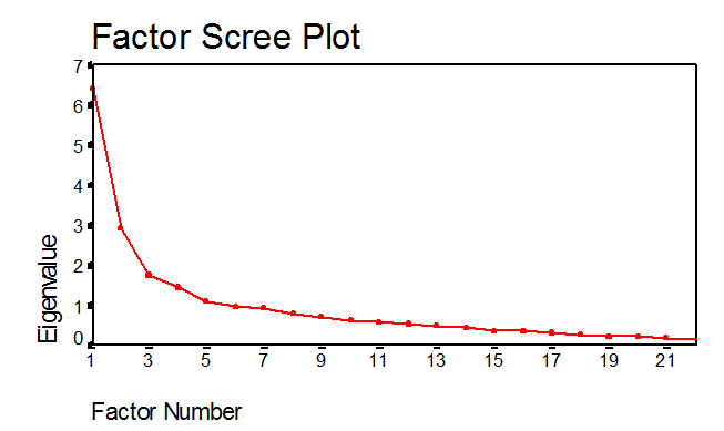
Another method
to assess the number of factors is to utilize the scree test. When using this method the eigenvalues and
the number of factors are plotted (see page 3) and then the point on the graph
that contains the largest bend (or smallest angle), or elbow is found. The lines drawn on the plot help determine
the elbow. The number of factors at the
elbow is the number of factors selected.
According to my judgement the elbow is at six factors. This indicates a different number of factors
would be selected using the methods of eigenvalues and the scree test. There were five selected by the eigenvalue
method and six selected using the scree test.
The next method
used to estimate the number of factors is the residual of the Reproduced
Matrix. The reproduced correlation
matrix can be thought of as Y'. The
reproduced matrix is much the same as the regression line in regression
analysis. In regression analysis the
difference between the regression line and the actual data is the
residual. In much the same way the
difference between the reproduced matrix and the actual correlation matrix is
the residual matrix. The residual
correlation matrix is the difference between the reproduced correlation matrix
and the actual correlation matrixes. If
the residual is great then it is probable that more factors exist. The reproduced and residual matrix
follow. The SPSS program presents the
reproduced matrix and the residual matrix as a single matrix. The reproduced matrix is below the diagonal
(the diagonal is identified by the asterisks) and the residual is above the the
diagonal.
Reproduced
Correlation Matrix:
LEISUR FEAR DEPRES FEELG ANGRY
LEISUR .54402* ‑.00782 ‑.00077 .01341 .05405
FEAR ‑.37492 .67085* ‑.00030 .07773 ‑.10014
DEPRES ‑.30041 .68663 .78216* .02137 ‑.03101
FEELG .45969 ‑.44708 ‑.35890 .62382* ‑.04192
ANGRY ‑.19559 .50465 .64136 ‑.23713 .60650*
CONFUS ‑.33521 .67179 .76030 ‑.37814 .62867
WORTH .47849 ‑.38364 ‑.26720 .62509 ‑.14593
TENSE ‑.26478 .57799 .68959 ‑.24302 .61008
USELES ‑.30504 .60194 .68233 ‑.27503 .53401
SATISF .48352 ‑.50056 ‑.41370 .63466 ‑.27192
OUTSID .42313 ‑.32244 ‑.18765 .29364 ‑.04233
BILLS .26871 ‑.23591 ‑.16382 .16242 .02426
TALKTO .56160 ‑.37474 ‑.29063 .36742 ‑.17295
CONFLT ‑.18168 .20461 .27533 ‑.33640 .34400
ALCDRG .08707 ‑.11465 .04902 .08876 .23660
SUPPRT .45522 ‑.22436 ‑.24935 .12123 ‑.23179
EMPLOY .21590 ‑.14971 ‑.12874 .08478 .01050
GOODJ .38102 ‑.12130 ‑.09278 .21051
‑.01827
LIKEW .36395 ‑.16013 ‑.11143 .35128 ‑.04283
INWAY ‑.11748 .38852 .53237 ‑.12589 .49920
MONEY .31472 ‑.10203 ‑.06622 .31027 ‑.02402
HEALTH .41395 ‑.02890 .01909 .24819 ‑.01276
CONFUS WORTH TENSE USELES SATISF
LEISUR ‑.03951 ‑.04084 .03204 .05399 ‑.09062
‑ ‑ ‑ ‑ ‑ ‑
‑ ‑ ‑ ‑ ‑
F A C T O R A N A L Y S I S ‑ ‑ ‑ ‑ ‑ ‑
‑ ‑ ‑ ‑ ‑
CONFUS WORTH TENSE USELES SATISF
FEAR ‑.01451 .08071 ‑.03204 ‑.04973 .01502
DEPRES ‑.04350 .01610 ‑.01789 ‑.01655 .06542
FEELG ‑.00497 ‑.04148 .01148 .03959 ‑.13432
ANGRY ‑.01211 ‑.03288 ‑.10691 ‑.03317 .02335
CONFUS .74488* .07308 ‑.05516 ‑.07898 ‑.00776
WORTH ‑.29337 .64667* ‑.01082 ‑.08542 ‑.10134
TENSE .67569 ‑.15078 .67305* ‑.03657 ‑.02719
USELES .66563 ‑.20691 .59688 .64230* .00866
SATISF ‑.43019 .63005 ‑.29482 ‑.32979 .65307*
OUTSID ‑.20484 .30520 ‑.21709 ‑.19300 .33847
BILLS ‑.16390 .19955 ‑.04505 ‑.27103 .19275
TALKTO ‑.32514 .38399 ‑.30750 ‑.32038 .40699
CONFLT .29359 ‑.30387 .24161 .16355 ‑.31856
ALCDRG .06443 .12024 .10723 .00601 .11943
SUPPRT ‑.28916 .12938 ‑.32761 ‑.32539 .15262
EMPLOY ‑.13284 .12585 ‑.00760 ‑.25948 .10264
GOODJ ‑.12688 .26814 ‑.01516 ‑.21430 .21405
LIKEW ‑.14251 .39981 ‑.00318 ‑.16379 .34389
INWAY .51771 ‑.05501 .47803 .47987 ‑.15279
MONEY ‑.09758 .35961 .03526 ‑.11821 .29597
HEALTH ‑.03572 .29830 ‑.02327 ‑.03104 .23936
OUTSID BILLS TALKTO CONFLT ALCDRG
LEISUR ‑.09550 .01767
‑.08995 ‑.05613 .01799
FEAR .04984 .08679 .04650 .00580 ‑.04204
DEPRES ‑.04181 .05128 .06454 ‑.02400 ‑.02455
FEELG ‑.07855 ‑.01019 .02317
.09534 ‑.01081
ANGRY ‑.02679 ‑.09272 ‑.05275 .01824 .01811
CONFUS .00723 .00184 ‑.02437 ‑.04959 .02899
WORTH ‑.01725 .06821 ‑.02467 .05680 ‑.07574
TENSE ‑.00162 .01325 .07063 ‑.03640 ‑.01375
USELES ‑.00934 .04255 .03739 ‑.01814 .03384
SATISF ‑.01829 .06886 .05338 .06763 ‑.09189
OUTSID .67907* ‑.06250 ‑.06109 ‑.07734 ‑.09166
BILLS .19681 .53963* .02275 .01195 ‑.16477
TALKTO .58397 .28410 .67310* .00206 ‑.08076
CONFLT .13773 .16809 ‑.03684 .51572* ‑.21630
ALCDRG .40004 .27938 .18652 .37280 .56859*
SUPPRT .35476 .22909 .57466 ‑.06280 ‑.09257
EMPLOY .00200 .54130 .18670 .10167 .10719
GOODJ .05554 .46326 .33412 ‑.07748 ‑.04424
LIKEW .02393 .34256 .25437 ‑.20967 ‑.05349
INWAY .10014 ‑.07637 ‑.07176 .26567 .25108
MONEY ‑.04726 .30042 .19118 ‑.22506 ‑.10521
HEALTH .21647 .11951 .41780 ‑.18775 ‑.12196
‑ ‑ ‑ ‑ ‑ ‑
‑ ‑ ‑ ‑ ‑
F A C T O R A N A L Y S I S ‑ ‑ ‑ ‑ ‑ ‑
‑ ‑ ‑ ‑ ‑
SUPPRT EMPLOY GOODJ LIKEW INWAY
LEISUR ‑.05672 .04548 .02828 ‑.16156 ‑.03462
FEAR ‑.05666 .06404 ‑.01395 ‑.05178 ‑.03942
DEPRES .01498 .02681 .00717 ‑.08974 ‑.05706
FEELG .05804 .02908 .05820
‑.04945 ‑.04759
ANGRY .03301 ‑.10424 .01162 .08488 ‑.16255
CONFUS .08079 .00500 ‑.03664 .05322 ‑.03431
WORTH .06541 .06018 ‑.09260 ‑.09048 ‑.03821
TENSE .03439 .00963 ‑.03448 ‑.07780 ‑.04373
USELES ‑.01187 .02342 .07584 ‑.04953 ‑.11002
SATISF ‑.00583 ‑.04770 ‑.00278 .05850 ‑.02243
OUTSID ‑.08589 .08700 .01232 .06223 .02232
BILLS ‑.04461 ‑.13493 ‑.09140 ‑.12137 ‑.02960
TALKTO ‑.04903 .00476 .00043 ‑.00286 ‑.04704
CONFLT ‑.04265 ‑.15094 ‑.07715 .10735 ‑.03604
ALCDRG .09860 ‑.02217 .07506 ‑.02158 ‑.10515
SUPPRT .73067* ‑.01150 ‑.06330 .04867 ‑.02774
EMPLOY .25564 .63235* ‑.03753 ‑.12263 .10704
GOODJ .43617 .57687 .68609* ‑.04256 .00302
LIKEW .24923 .42372 .54894 .53001* .07141
INWAY ‑.20071 ‑.15131 ‑.14105 ‑.11450 .48184*
MONEY .21454 .40207 .53247 .51775 ‑.10759
HEALTH .47078 .15739 .41231 .35589 .00567
MONEY HEALTH
LEISUR ‑.07053 ‑.03668
FEAR ‑.07562 ‑.03057
DEPRES ‑.02862 ‑.06952
FEELG ‑.10712 ‑.05348
ANGRY .01770 ‑.00718
CONFUS ‑.02686 ‑.05252
WORTH ‑.04691 .00223
TENSE ‑.00749 ‑.03086
USELES ‑.01887 ‑.04896
SATISF ‑.04809 ‑.00184
OUTSID .09746 ‑.04987
BILLS ‑.10613 .09877
TALKTO .00710 ‑.16746
CONFLT .06275 .11376
ALCDRG .06525 .07363
SUPPRT .00238 ‑.14548
EMPLOY ‑.08578 ‑.06075
GOODJ ‑.12418 ‑.05984
LIKEW ‑.03554 ‑.05722
INWAY ‑.00336 .00321
‑ ‑ ‑ ‑ ‑ ‑
‑ ‑ ‑ ‑ ‑
F A C T O R A N A L Y S I S ‑ ‑ ‑ ‑ ‑ ‑
‑ ‑ ‑ ‑ ‑
MONEY HEALTH
MONEY .51483* ‑.00802
HEALTH .34407 .52015*
The
lower left triangle contains the reproduced correlation matrix; the
diagonal,
reproduced communalities; and the upper right triangle residuals
between
the observed correlations and the reproduced correlations.
There
are 97 (41.0%) residuals (above
diagonal) with absolute values > 0.05.
There are 97 (41.0%) residuals (above diagonal) that
are > 0.05
The reproduced correlation
matrix can be used to determine the number of factors. If the actual matrix is not much different
from the reproduced correlation matrix then no more factors are needed. However, if the actual matrix is different
from the reproduced correlation matrix then more factors are needed. The question is how much different is
different. Tabachnick and Fidell (1989)
say "Several moderate residuals (say, .05 to .10) or a few large residuals
(say > .10) suggest the presence of another factor" (p. 636). It looks to me like there are more factors
here.
Consequently, both the
scree test and the reproduced correlation matrix indicate that there are more
than five factors, while the eigenvalue method indicates that there are five
factors. The next method used to
identify the number of factors is interpretability of the factor structure. The Rotated Factor Matrix is used for interpretability. A variable of .60 is said to load a factor ‑‑
these are marked on the printout by check marks (done manually). The factor structure is then scanned for
interpretability. The interpretation is
up to you. If the interpretation doesn't
make sense to you then try adding or deleting a factor and then assessing the
new factor structure for interpretation.
The interpretation is determined by your theory. It should be remembered that this is
exploratory factor analysis and you are searching for the underlying factors
that you will test with confirmatory factory analysis. You are at the exploratory or descriptive
level of analysis. You are not testing
theory ‑‑ you are generating theory.
VARIMAX rotation
1 for extraction 1 in
analysis 1 ‑ Kaiser Normalization.
VARIMAX
converged in 8 iterations.
Rotated
Factor Matrix:
Factor 1
Factor 2 Factor
3 Factor 4
Factor 5
LEISUR ‑.20373 .44057 .23534 .49753 .07410
FEAR .70024 ‑.36192 ‑.07026 ‑.08428 ‑.19360
DEPRES .85664 ‑.20974 ‑.04572 ‑.04254 ‑.02103
FEELG ‑.22569 .73830 .11217 .12185 .01906
ANGRY .72939 ‑.10369 .07609 ‑.07280 .22944
CONFUS .82189 ‑.23522 ‑.06025 ‑.10171 .00864
WORTH ‑.10764 .76014 .17883 .15410 .03929
TENSE .78356 ‑.07347 .10739 ‑.20229 .03505
USELES .75596 ‑.08895 ‑.20688 ‑.11445 ‑.08369
SATISF ‑.28965 .72821 .11357 .14385 .07271
OUTSID ‑.11797 .27901 ‑.13013 .53764 .53040
BILLS ‑.12962 .06371 .61115 .08623 .37126
TALKTO ‑.22089 .29043 .14186 .67719 .24747
CONFLT .23811 ‑.40072 .03801 ‑.01195 .54485
ALCDRG .10834 .13410 .02336 ‑.01966 .73344
SUPPRT ‑.26022 ‑.07924 .25685 .76615 ‑.06094
EMPLOY ‑.11523 ‑.04834 .76992 .04324 .14864
GOODJ ‑.02716 .11335 .75268 .31209 ‑.09264
LIKEW ‑.00584 .36309 .59347 .14972 ‑.15335
INWAY .62915 .03398 ‑.14965 .02518
.24863
MONEY .03459 .32926 .58512 .11182 ‑.22441
HEALTH .11883 .24491 .24769 .57954 ‑.22097
‑ ‑ ‑ ‑ ‑ ‑
‑ ‑ ‑ ‑ ‑
F A C T O R A N A L Y S I S ‑ ‑ ‑ ‑ ‑ ‑
‑ ‑ ‑ ‑ ‑
Factor
Transformation Matrix:
Factor 1
Factor 2 Factor
3 Factor 4
Factor 5
Factor 1
‑.68846 .50289 .34249 .39409 .02260
Factor 2
.66556 .22494 .59779 .34637 .17059
Factor 3
.05869 .20689 ‑.50701 .23318 .80145
Factor 4
.27410 .74769 ‑.40353 ‑.09937 ‑.43945
Factor 5
.06687 ‑.30767 ‑.32473 .81270
‑.36735
Factor
Score Coefficient Matrix:
Factor 1
Factor 2 Factor
3 Factor 4
Factor 5
LEISUR .02865 .09648 ‑.01583 .19438 .00312
FEAR .15520 ‑.08401 .00424 .09475 ‑.13821
DEPRES .21439 .00594 ‑.00382 .08390 ‑.04171
FEELG .03559 .33975 ‑.04032 ‑.09311 .00157
ANGRY .17791 .03748 .05959 ‑.01488 .12632
CONFUS .19596 ‑.00016 .00374 .04486 ‑.01547
WORTH .07252 .35325 ‑.01645 ‑.08052 .00780
TENSE .19488 .08428 .08904 ‑.09072 .01614
USELES .20015 .09018 ‑.08325 .04039 ‑.07584
SATISF .01568 .32126 ‑.04024 ‑.08676 .03572
OUTSID .02164 .04342 ‑.17379 .27669 .27372
BILLS ‑.04452 ‑.06598 .29109 ‑.11279 .24681
TALKTO .01243 ‑.01372 ‑.07364 .34344 .09304
CONFLT ‑.00608 ‑.19773 .07578 .01954 .34085
ALCDRG .01624 .07813 .02161
‑.11253 .45788
SUPPRT ‑.02741 ‑.24466 ‑.00355 .48250 ‑.10039
EMPLOY ‑.05061 ‑.13075 .38194 ‑.12571 .11699
GOODJ .02441 ‑.07668 .29952 .06439 ‑.06947
LIKEW .05405 .10984 .22274 ‑.05697 ‑.09936
INWAY .17597 .10488 ‑.08190 .05850 .12350
MONEY .06140 .10535 .22646 ‑.06469 ‑.14145
HEALTH .11321 .01757 ‑.01697 .34028 ‑.20112
‑ ‑ ‑ ‑ ‑ ‑
‑ ‑ ‑ ‑ ‑
F A C T O R A N A L Y S I S ‑ ‑ ‑ ‑ ‑ ‑
‑ ‑ ‑ ‑ ‑
Covariance
Matrix for Estimated Regression Factor Scores:
Factor 1
Factor 2 Factor
3 Factor 4
Factor 5
Factor 1
1.00000
Factor 2
.00000 1.00000
Factor 3
.00000 .00000 1.00000
Factor 4
.00000 .00000 .00000 1.00000
Factor 5
.00000 .00000 .00000 .00000 1.00000
This next analysis was computed because the
reproduced correlation matrix, the scree test, and the interpretability of the
Rotated Factor Matrix all indicated that there may be more factors. Much of the printout has been deleted to save
space.
|
File Name = crsfac3.sps
|
|
get file = '\rdda\crsleq9.sav'.
MISSING VALUES GROUP TO HEALTH (9).
FACTOR VAR = LEISUR TO HEALTH
/MISSING = PAIRWISE
/CRITERIA = FACTORS(6)
/PRINT = INITIAL EXTRACTION ROTATION REPR FSCORE
/PLOT = EIGEN
/ ROTATION.
|
[EXTRACTION STATISTICS WERE
ELIMINATED TO SAVE SPACE.]
‑ ‑ ‑ ‑ F A C T O R
A N A L Y S I S ‑ ‑ ‑
‑
Final
Statistics:
Variable Communality *
Factor Eigenvalue Pct of Var
Cum Pct
*
LEISUR .65313 *
1 6.39831 29.1 29.1
FEAR .67336 * 2
2.91594 13.3 42.3
DEPRES .78759 *
3 1.74551 7.9 50.3
FEELG .64446 *
4 1.47050 6.7 57.0
ANGRY .61885 *
5 1.12909 5.1 62.1
CONFUS .74497 *
6 .95818 4.4 66.4
WORTH .64699 *
TENSE .68648 *
USELES .66751 *
SATISF .70785 *
OUTSID .68074 *
BILLS .55247 *
TALKTO .67310 *
CONFLT .75824 *
ALCDRG .65774 *
SUPPRT .73404 *
EMPLOY .73476 *
GOODJ .72702 *
LIKEW .67981 *
INWAY .48596 *
MONEY .54224 *
HEALTH .56022 *
[REPRODUCED CORRELATION MATRIX IS
ELIMINATED TO SAVE SPACE.]
The lower left triangle contains
the reproduced correlation matrix; The
diagonal, communalities; and the upper right triangle, residuals between the
observed correlations and the reproduced correlations.
There are 89 (38.0%) residuals (above diagonal) that
are > 0.05
Page 9 SPSS/PC+ 2/11/91
‑ ‑ ‑ ‑ F A C T O R
A N A L Y S I S ‑ ‑ ‑
‑
Varimax Rotation
1, Extraction 1,
Analysis 1 ‑ Kaiser
Normalization.
Varimax converged in 10 iterations.
Rotated
Factor Matrix:
FACTOR 1 FACTOR 2
FACTOR 3 FACTOR
4 FACTOR 5
LEISUR ‑.18100 .36760 .28070 .51699 .19517
FEAR .70292 ‑.35918 ‑.06504 ‑.11076 ‑.18009
DEPRES .86149 ‑.20130 ‑.03651 ‑.05248 ‑.02605
FEELG ‑.22346 .68596 .10018 .13987 .13566
ANGRY .72468 ‑.03284 .05766 ‑.06384 .08482
CONFUS .82145 ‑.20706 ‑.06359 ‑.11092 ‑.03700
WORTH ‑.11638 .75455 .12858 .16833 .05206
TENSE .79056 ‑.05940 .11875 ‑.20422 .04623
USELES .76311 ‑.12623 ‑.18510 ‑.12285 .01441
SATISF ‑.31240 .76267 .02809 .15716 ‑.01360
OUTSID ‑.11394 .28447 ‑.11166 .58765 .42373
BILLS ‑.12839 .16853 .59655 .11128 .15149
TALKTO ‑.21605 .29450 .14204 .70110 .15604
CONFLT .21716 ‑.23397 ‑.00753 .01401 .14851
ALCDRG .13823 .10998 .12809 .05332 .76745
SUPPRT ‑.24972 ‑.08403 .26759 .75712 ‑.12800
EMPLOY ‑.08518 ‑.03248 .83247 .05644 .15515
GOODJ ‑.01002 .13319 .76133 .30220 ‑.11663
LIKEW ‑.03576 .49009 .46255 .12586 ‑.40664
INWAY .62566 .06257 ‑.15702 .04207 .17084
MONEY .01906 .40407 .49702 .08676 ‑.35220
HEALTH .10250 .29036 .16468 .55318 ‑.36366
FACTOR 6
LEISUR ‑.31793
FEAR ‑.03633
DEPRES .01151
FEELG ‑.27565
ANGRY .27932
CONFUS .09799
WORTH ‑.12856
TENSE ‑.00523
USELES ‑.14030
SATISF .05404
OUTSID .22244
BILLS .34115
TALKTO .06018
CONFLT .79626
ALCDRG .13528
SUPPRT ‑.05828
EMPLOY ‑.07860
GOODJ ‑.15692
LIKEW .20782
INWAY .18702
MONEY .00213
‑ ‑ ‑ ‑ F A C T O R
A N A L Y S I S ‑ ‑ ‑
‑
HEALTH .00502
Factor
Transformation Matrix:
FACTOR 1
FACTOR 2 FACTOR
3 FACTOR 4 FACTOR
FACTOR 1
‑.68898 .49903 .31876 .40504 .00201
FACTOR 2
.66865 .30381 .56509 .35192 ‑.00039
FACTOR 3
.06642 .19034 ‑.44923 .31046 .74619
FACTOR 4
.25375 .66328 ‑.47639 ‑.12282 ‑.23451
FACTOR 5
.06781 ‑.36265 ‑.32584 .77458 ‑.35405
FACTOR 6
‑.06944 .22579 ‑.21009 ‑.02555 ‑.51269
FACTOR 6
FACTOR 1
‑.10299
FACTOR 2
.13203
FACTOR 3
.32306
FACTOR 4
‑.44570
FACTOR 5
‑.17996
FACTOR 6
.79785
Factor
Score Coefficient Matrix:
FACTOR
1 FACTOR 2
FACTOR 3 FACTOR
4 FACTOR 5
LEISUR .05223 .01187 .05052 .20417 .17182
FEAR .15797 ‑.09757 .00672 .08083 ‑.11188
DEPRES .21889 ‑.00977 .00425 .08022 ‑.01140
FEELG .04062 .29252 ‑.02920 ‑.08286 .12190
ANGRY .17107 .08106 .03655 ‑.00818 .03201
CONFUS .19478 .00632 ‑.00394 .04139 ‑.03161
WORTH .06586 .34736 ‑.04260 ‑.07441 .03500
TENSE .20188 .07113 .10379 ‑.08692 .06716
USELES .20850 .04142 ‑.06168 .03854 .03116
SATISF ‑.00581 .36501 ‑.10789 ‑.08378 ‑.05315
OUTSID .02275 .04546 ‑.16152 .30066 .21293
BILLS ‑.04691 .00842 .28139 ‑.09748 .10182
TALKTO .01533 ‑.01991 ‑.06500 .35044 .05616
CONFLT ‑.03334 ‑.04784 .00276 .03205 ‑.01202
ALCDRG .04330 .03576 .11467 ‑.06307 .55298
SUPPRT ‑.01876 ‑.26389 .01721 .46927 ‑.11558
EMPLOY ‑.02226 ‑.15407 .45947 ‑.11211 .20618
GOODJ .04103 ‑.09421 .33480 .05885 ‑.01361
LIKEW .02381 .21757 .11671 ‑.07660 ‑.31475
INWAY .17118 .11884 ‑.09517 .06849 .07808
MONEY .04659 .15932 .16595 ‑.08224 ‑.23189
HEALTH .09685 .04901 ‑.07887 .31540 ‑.30557
FACTOR 6
LEISUR ‑.30066
FEAR ‑.09167
DEPRES ‑.07826
FEELG ‑.19922
ANGRY .16727
CONFUS .00763
WORTH ‑.06030
TENSE ‑.08648
USELES ‑.19626
SATISF .13713
OUTSID .14643
BILLS .27816
TALKTO .03946
CONFLT .64885
ALCDRG ‑.01339
SUPPRT ‑.05762
EMPLOY ‑.12705
GOODJ ‑.15309
LIKEW .27280
INWAY .09257
MONEY .06757
HEALTH .04936
This solution looks pretty good. The scree test indicated that there were six
factors and the interpretation is adequate according to my theory. First the psychological distress factor made
up of FEAR, DEPRES, ANGRY, CONFUS, TENSE, USELES, and INWAY are what I had in
mind for this test. The Quality of Life
factor of FEELG, WORTH, and SATISF is intact (although LEISUR is missing). The Employment Factor of BILLS, EMPLOY, and
GOODJ are on target. The Relationship
factor of OUTSID, TALKTO, and SUPPRT holds together nicely. The single variable factors of ALCDRG
(alcohol and drugs), and CONFLT seem separate.
However, another analysis of seven factors is computed just to see if
there might be more factors.
|
File Name = crsfac6.sps
|
|
get file = '\rdda\crsleq9.sav'.
MISSING VALUES GROUP TO HEALTH (9).
FACTOR VAR = LEISUR TO HEALTH
/MISSING = PAIRWISE
/CRITERIA = FACTORS(7)
/PRINT = INITIAL EXTRACTION ROTATION REPR FSCORE
/PLOT = EIGEN
/ ROTATION.
|
Final
Statistics:
Variable Communality *
Factor Eigenvalue Pct of Var
Cum Pct
*
LEISUR .66151 *
1 6.39831 29.1 29.1
FEAR .74712 *
2 2.91594 13.3 42.3
DEPRES .80420 *
3 1.74551 7.9 50.3
FEELG .66305 *
4 1.47050 6.7 57.0
ANGRY .69795 *
5 1.12909 5.1 62.1
CONFUS .74990 *
6 .95818 4.4 66.4
WORTH .69373 *
7 .93068 4.2 70.7
TENSE .69631 *
USELES .66785 *
SATISF .71178 *
OUTSID .68983 *
BILLS .79704 *
TALKTO .68976 *
CONFLT .78558 *
ALCDRG .80696 *
SUPPRT .75630 *
EMPLOY .74054 *
GOODJ .73465 *
LIKEW .78069 *
INWAY .48623 *
MONEY .61946 *
HEALTH .56783 *
Reproduced
Correlation Matrix:
LEISUR FEAR DEPRES
FEELG ANGRY
LEISUR .66151* ‑.04921 ‑.03692 ‑.04653 .11650
FEAR ‑.33353 .74712* ‑.03899 .03351 ‑.01819
DEPRES ‑.26427 .72532 .80420* ‑.00679 .01343
FEELG .51963 ‑.40287 ‑.33074 .66305* .01239
ANGRY ‑.25804 .42270 .59693 ‑.29144 .69795*
CONFUS ‑.34479 .65225 .75055 ‑.38908 .64947
WORTH .49237 ‑.32582 ‑.24065 .65199 ‑.20474
TENSE ‑.21743 .61071 .71091 ‑.21286 .56932
USELES ‑.25090 .61488 .69641 ‑.24971 .51119
SATISF .41193 ‑.49527 ‑.42289 .60957 ‑.26352
OUTSID .40092 ‑.35038 ‑.20295 .27478 ‑.01098
BILLS .27653 ‑.10727 ‑.10845 .21356 ‑.10223
TALKTO .57283 ‑.33977 ‑.27413 .38476 ‑.20906
CONFLT ‑.32922 .22486 .26032 ‑.38462 .35224
ALCDRG .15035 ‑.20462 .02125 .07900 .31206
SUPPRT .46075 ‑.26197 ‑.26429 .10924 ‑.19628
EMPLOY .32856 ‑.11305 ‑.09536 .14112 ‑.04644
GOODJ .43985 ‑.13489 ‑.08913 .22767 ‑.01619
LIKEW .20704 ‑.26577 ‑.18090 .25237 .08951
INWAY ‑.13719 .38975 .52975 ‑.13288 .50173
MONEY .23461 ‑.18580 ‑.11423 .24860 .07254
HEALTH .35581 ‑.01523 .01558 .23132 ‑.01505
Page
7
SPSS/PC+
2/11/91
‑ ‑ ‑ ‑ F A C T O R
A N A L Y S I S ‑ ‑ ‑
‑
CONFUS WORTH TENSE USELES SATISF
LEISUR ‑.02993 ‑.05472 ‑.01531 ‑.00015 ‑.01903
FEAR .00503 .02289 ‑.06476 ‑.06268 .00973
DEPRES ‑.03375 ‑.01044 ‑.03920 ‑.03063 .07461
FEELG .00597 ‑.06838 ‑.01868 .01427 ‑.10922
ANGRY ‑.03291 .02594 ‑.06615 ‑.01035 .01494
CONFUS .74990* .08808 ‑.04710 ‑.07617 ‑.00560
WORTH ‑.30837 .69373* ‑.03017 ‑.08655 ‑.11906
TENSE .66763 ‑.13143 .69631* ‑.05680 ‑.00626
USELES .66282 ‑.20577 .61711 .66785* .04468
SATISF ‑.43235 .64777 ‑.31574 ‑.36580 .71178*
OUTSID ‑.19776 .28532 ‑.23126 ‑.20124 .34206
BILLS ‑.19753 .30848 ‑.00917 ‑.27993 .25023
TALKTO ‑.33419 .41192 ‑.29492 ‑.31829 .41549
CONFLT .28668 ‑.25932 .20091 .08839 ‑.19294
ALCDRG .08869 .03139 .10355 .04631 .02536
SUPPRT ‑.27924 .09608 ‑.33567 ‑.31892 .12969
EMPLOY ‑.14123 .13655 .03703 ‑.20727 .03250
GOODJ ‑.12268 .24564 ‑.00037 ‑.18378 .16123
LIKEW ‑.11652 .33806 ‑.07952 ‑.23109 .41459
INWAY .51717 ‑.05032 .47221 .46997 ‑.13673
MONEY ‑.07650 .30250 ‑.01147 ‑.14960 .31732
HEALTH ‑.03993 .32074 ‑.03782 ‑.06122 .29168
OUTSID BILLS TALKTO CONFLT ALCDRG
LEISUR ‑.07329 .00985 ‑.10118 .09142 ‑.04529
FEAR .07777 ‑.04185 .01153 ‑.01445 .04793
DEPRES ‑.02651 ‑.00409 .04804 ‑.00900 .00321
FEELG ‑.05969 ‑.06132 .00583 .14356 ‑.00105
ANGRY ‑.05814 .03377 ‑.01665 .01000 ‑.05734
CONFUS .00015 .03547 ‑.01533 ‑.04269 .00473
WORTH .00263 ‑.04073 ‑.05260 .01225 .01311
TENSE .01256 ‑.02262 .05805 .00430 ‑.01008
USELES ‑.00111 .05145 .03529 .05702 ‑.00646
SATISF ‑.02187 .01137 .04489 ‑.05799 .00218
OUTSID .68983* ‑.01997 ‑.04886 ‑.08168 ‑.11630
BILLS .15429 .79704* ‑.04127 ‑.12562 .06010
TALKTO .57174 .34813 .68976* ‑.02015 ‑.03038
CONFLT .14207 .30566 ‑.01463 .78558* ‑.00540
ALCDRG .42468 .05451 .13614 .16190 .80696*
SUPPRT .36661 .14872 .55530 ‑.11606 ‑.01760
EMPLOY ‑.01831 .54262 .19594 ‑.04336 .17339
GOODJ .05561 .39713 .32249 ‑.19155 .04990
LIKEW .07000 .22935 .21406 ‑.07158 ‑.04636
INWAY .10120 ‑.06100 ‑.06953 .30000 .22558
MONEY ‑.01401 .18175 .15561 ‑.18948 ‑.04730
HEALTH .21632 .18534 .42941 ‑.07475 ‑.21542
SUPPRT EMPLOY GOODJ LIKEW INWAY
LEISUR ‑.06225 ‑.06719 ‑.03055 ‑.00464 ‑.01490
FEAR ‑.01904 .02738 ‑.00035 .05387 ‑.04065
DEPRES .02993 ‑.00658 .00352 ‑.02028 ‑.05444
FEELG .07004 ‑.02726 .04104 .04946 ‑.04059
ANGRY ‑.00250 ‑.04730 .00954 ‑.04747 ‑.16508
CONFUS .07087 .01339 ‑.04084 .02723 ‑.03377
WORTH .09871 .04948 ‑.07010 ‑.02873 ‑.04289
TENSE .04244 ‑.03500 ‑.04928 ‑.00146 ‑.03791
USELES ‑.01835 ‑.02880 .04533 .01776 ‑.10013
SATISF .01711 .02245 .05004 ‑.01221 ‑.03848
OUTSID ‑.09774 .10730 .01225 .01615 .02125
BILLS .03576 ‑.13624 ‑.02528 ‑.00815 ‑.04498
TALKTO ‑.02967 ‑.00449 .01206
.03746 ‑.04927
CONFLT .01062 ‑.00591 .03691 ‑.03074 ‑.07037
ALCDRG .02363 ‑.08837 ‑.01908 ‑.02872 ‑.07966
SUPPRT .75630* ‑.01875 ‑.08808 .02376 ‑.02157
EMPLOY .26288 .74054* ‑.09563 .02536 .12634
GOODJ .46095 .63497 .73465* .00799 .01744
LIKEW .27415 .27573 .49838 .78069* .05175
INWAY ‑.20688 ‑.17062 ‑.15547 ‑.09485 .48623*
MONEY .24639 .32798 .52326 .67008 ‑.10151
HEALTH .44614 .09996 .36420 .40565 .01995
MONEY HEALTH
LEISUR .00958 .02146
FEAR .00814 ‑.04424
DEPRES .01939 ‑.06600
FEELG ‑.04545 ‑.03661
ANGRY ‑.07886 ‑.00489
CONFUS ‑.04795 ‑.04831
WORTH .01021 ‑.02021
TENSE .03924 ‑.01631
USELES .01253 ‑.01878
SATISF ‑.06944 ‑.05415
OUTSID .06421 ‑.04972
BILLS .01254 .03295
TALKTO .04267 ‑.17907
CONFLT .02716 .00076
ALCDRG .00734 .16710
SUPPRT ‑.02947 ‑.12084
EMPLOY ‑.01169 ‑.00333
GOODJ ‑.11497 ‑.01173
LIKEW ‑.18787 ‑.10698
INWAY ‑.00944 ‑.01107
MONEY .61946* ‑.01692
HEALTH .35297
.56783*
The
lower left triangle contains the reproduced correlation matrix; The
diagonal,
communalities; and the upper right triangle, residuals between
the
observed correlations and the reproduced correlations.
There
are 63 (27.0%) residuals (above
diagonal) that are > 0.05
‑ ‑ ‑ ‑ F A C T O R
A N A L Y S I S ‑ ‑ ‑
‑
Varimax Rotation
1, Extraction 1,
Analysis 1 ‑ Kaiser
Normalization.
Varimax converged in 10 iterations.
Rotated
Factor Matrix:
FACTOR 1
FACTOR 2 FACTOR
3 FACTOR 4
FACTOR 5
LEISUR ‑.16673 .45967 .50509 .02141 .30917
FEAR .72932 ‑.26424 ‑.08939 ‑.17865 .02616
DEPRES .87197 ‑.16249 ‑.04497 ‑.08336 .00373
FEELG ‑.21110 .73741 .11227 .08825 .10164
ANGRY .68760 ‑.19173 ‑.07236 .24388 ‑.07400
CONFUS .81085 ‑.25907 ‑.10549 .03590 ‑.09333
WORTH ‑.10386 .78945 .13805 .17249 .09731
TENSE .79636 ‑.04370 ‑.20192 .00795 .13648
USELES .76854 ‑.10150 ‑.11996 ‑.12074 ‑.13953
SATISF ‑.31899 .70867 .12316 .28126 ‑.07640
OUTSID ‑.12450 .28952 .55241 ‑.06497 ‑.12512
BILLS ‑.09572 .29640 .10494 .03808 .64624
TALKTO ‑.20674 .35996 .68350 .02050 .13882
CONFLT .21541 ‑.24603 .00354 ‑.06221 ‑.01559
ALCDRG .10679 .05324 .01999 ‑.05907 .11886
SUPPRT ‑.26278 ‑.11730 .77020 .19610 .18213
EMPLOY ‑.07931 .00663 .07054 .18889 .82574
GOODJ ‑.02396 .06862 .31704 .44905 .63270
LIKEW ‑.09005 .20030 .12104 .83490 .12644
INWAY .62184 .05325 .02505 ‑.04876 ‑.15850
MONEY ‑.02397 .17444
.08881 .71887 .22434
HEALTH .09885 .24291 .55448 .34364 .03771
FACTOR 6
FACTOR 7
LEISUR .12521 ‑.23575
FEAR ‑.32128 .03969
DEPRES ‑.07968 .04611
FEELG .07185 ‑.19703
ANGRY .30175 .16478
CONFUS .03230 .05595
WORTH ‑.00202 ‑.03783
TENSE .00890 .02567
USELES ‑.01328 ‑.13517
SATISF .04685 .07414
OUTSID .46853 .21436
BILLS ‑.06122 .51594
TALKTO .11786 .12916
CONFLT .12410 .81186
ALCDRG .87872 .05057
SUPPRT ‑.00461 ‑.09292
EMPLOY .10691 ‑.01668
GOODJ .00237 ‑.16397
LIKEW ‑.02146 .06559
INWAY .18484 .18552
MONEY ‑.03924 ‑.10916
HEALTH ‑.26770 .02087
According to the Reproduced Correlation
Matrix this may be the best solution ‑‑ the number of residual
correlations that are significant is below 30% (maybe that is a few). This last solution did not help my
interpretation very much. It essentially
split the Employment Factor into two factors.
I think they should remain as a single factor.
This next section is an extended method
that is not much used and rather involved and consequently may be
bypassed. It shows two things: (1) how
you can use the Factor Score Coefficients to create a factor score for a specific individual, and
(2) how you could use the coefficients to score a subtest that is based on
factor scores.
The coefficients are beta weights that can
be used to create Y' for a specific individual on a particular factor. The weights are multiplied by the z‑score
of the individual on a particular and the Factor Score Coefficient for that
factor and that variables. Consequently,
the predicted factor score on Factor 1 would be:
The Y' does not contain the constant
because it is in standardized form and consequently the values of the data must
be in standard score format. That is the
actual values must first be changed into z‑scores. In order to obtain z‑scores you need
the mean and standard deviation of each variable. These can be obtained for the above data by
running the following program.
|
File Name = crsdes1.sps
|
|
get file ='\rdda\crsleq9.sav'.
MISSING VALUES GROUP TO HEALTH (9).
des var = leisur to health
/statistics=1 5.
DESCRIPTIVES
VARIABLES=leisur to health
/FORMAT=LABELS NOINDEX
/STATISTICS=MEAN STDDEV.
|
Variable Mean
Std Dev N Label
LEISUR 4.41 2.33
209
FEAR 3.08 2.77
212
DEPRES 4.15 2.68
207
FEELG 4.15 2.40
210
ANGRY 4.00 2.48
209
CONFUS 3.97 2.86
213
WORTH 4.33 2.58
211
TENSE 4.00 2.59
212
USELES 3.66 2.74
210
SATISF 4.21 2.33
206
OUTSID 4.35 2.56
208
BILLS 4.66 2.76
202
TALKTO 3.89
2.30 207
CONFLT 3.02 2.64
201
ALCDRG 2.08 2.51
205
SUPPRT 5.00 2.47
210
EMPLOY 5.08 3.36
201
GOODJ 5.28 2.65
202
LIKEW 4.89 2.46
199
INWAY 4.16
2.92 200
MONEY 5.26 3.01
196
HEALTH 5.35 2.40
211
The other values that are needed
are the Fscores the SPSS output. The
Fscores from the six factor solution above ‑‑ they are repeated
below.
Factor Score Coefficient
Matrix:
FACTOR
1 FACTOR 2
FACTOR 3 FACTOR
4 FACTOR 5
FACTOR 6
LEISUR .05223
.01187 .05052 .20417
.17182 ‑.30066
FEAR .15797
‑.09757 .00672 .08083
‑.11188 ‑.09167
DEPRES .21889
‑.00977 .00425 .08022
‑.01140 ‑.07826
FEELG .04062
.29252 ‑.02920 ‑.08286 .12190
‑.19922
ANGRY .17107
.08106 .03655 ‑.00818 .03201
.16727
CONFUS .19478
.00632 ‑.00394 .04139
‑.03161 .00763
WORTH .06586
.34736 ‑.04260 ‑.07441 .03500
‑.06030
TENSE .20188
.07113 .10379 ‑.08692 .06716
‑.08648
USELES .20850
.04142 ‑.06168 .03854
.03116 ‑.19626
SATISF ‑.00581 .36501
‑.10789 ‑.08378 ‑.05315 .13713
OUTSID .02275
.04546 ‑.16152 .30066
.21293 .14643
BILLS ‑.04691 .00842
.28139 ‑.09748 .10182
.27816
TALKTO .01533
‑.01991 ‑.06500 .35044
.05616 .03946
CONFLT ‑.03334 ‑.04784 .00276
.03205 ‑.01202 .64885
ALCDRG .04330
.03576 .11467 ‑.06307 .55298
‑.01339
SUPPRT ‑.01876 ‑.26389 .01721
.46927 ‑.11558 ‑.05762
EMPLOY ‑.02226 ‑.15407 .45947
‑.11211 .20618 ‑.12705
GOODJ .04103
‑.09421 .33480 .05885
‑.01361 ‑.15309
LIKEW .02381
.21757 .11671 ‑.07660 ‑.31475 .27280
INWAY .17118
.11884 ‑.09517 .06849
.07808 .09257
MONEY .04659
.15932 .16595 ‑.08224 ‑.23189 .06757
HEALTH .09685
.04901 ‑.07887 .31540
‑.30557 .04936
The next jobstream
performs three function: (1) computes the z‑score, (2) multiplies the
computed z‑score times the fscore and sums the values for each case, and
(3) lists the factor scores for the first five cases on factors 1, 2, and 5.
|
get file =
'\rdda\crsleq9.sav'.
MISSING VALUES GROUP TO HEALTH
(9).
compute ZLEISUR = ((LEISUR ‑
4.41 ) / 2.33).
compute ZFEAR = ((FEAR
‑ 3.08 ) / 2.77).
compute ZDEPRES = ((DEPRES ‑
4.15 ) / 2.68).
compute ZFEELG = ((FEELG
‑ 4.15 ) / 2.40).
compute ZANGRY = ((ANGRY
‑ 4.00 ) / 2.48).
compute ZCONFUS = ((CONFUS ‑
3.97 ) / 2.86).
compute ZWORTH = ((WORTH
‑ 4.33 ) / 2.58).
compute ZTENSE = ((TENSE
‑ 4.00 ) / 2.59).
compute ZUSELES = ((USELES ‑
3.66 ) / 2.74).
compute ZSATISF = ((SATISF ‑
4.21 ) / 2.33).
compute ZOUTSID = ((OUTSID ‑
4.35 ) / 2.56).
compute ZBILLS = ((BILLS
‑ 4.66 ) / 2.76).
compute ZTALKTO = ((TALKTO ‑
3.89 ) / 2.30).
compute ZCONFLT = ((CONFLT ‑
3.02 ) / 2.64).
compute ZALCDRG = ((ALCDRG ‑
2.08 ) / 2.51).
compute ZSUPPRT = ((SUPPRT ‑
5.00 ) / 2.47).
compute ZEMPLOY = ((EMPLOY ‑
5.08 ) / 3.36).
compute ZGOODJ = ((GOODJ
‑ 5.28 ) / 2.65).
compute ZLIKEW = ((LIKEW
‑ 4.89 ) / 2.46).
compute ZINWAY = ((INWAY
‑ 4.16 ) / 2.92).
compute ZMONEY = ((MONEY
‑ 5.26 ) / 3.01).
compute ZHEALTH = ((HEALTH ‑
5.35 ) / 2.40).
COMPUTE FACT1 =ZLEISUR * .05223.
COMPUTE FACT1 = FACT1 +
(ZFEAR * .15797).
COMPUTE FACT1 = FACT1 +
(ZDEPRES * .21889).
COMPUTE FACT1 = FACT1 +
(ZFEELG * .04062).
COMPUTE FACT1 = FACT1 +
(ZANGRY * .17107).
COMPUTE FACT1 = FACT1 +
(ZCONFUS * .19478).
COMPUTE FACT1 = FACT1 +
(ZWORTH * .06586).
COMPUTE FACT1 = FACT1 + (ZTENSE *
.20188).
COMPUTE FACT1 = FACT1 +
(ZUSELES * .20850).
COMPUTE FACT1 = FACT1 +
(ZSATISF * ‑.00581).
COMPUTE FACT1 = FACT1 +
(ZOUTSID * .02275).
COMPUTE FACT1 = FACT1 +
(ZBILLS * ‑.04691).
COMPUTE FACT1 = FACT1 +
(ZTALKTO * .01533).
COMPUTE FACT1 = FACT1 +
(ZCONFLT * ‑.03334).
COMPUTE FACT1 = FACT1 +
(ZALCDRG * .04330).
COMPUTE FACT1 = FACT1 +
(ZSUPPRT * ‑.01876).
COMPUTE FACT1 = FACT1 +
(ZEMPLOY * ‑.02226).
COMPUTE FACT1 = FACT1 +
(ZGOODJ * .04103).
COMPUTE FACT1 = FACT1 +
(ZLIKEW * .02381).
COMPUTE FACT1 = FACT1 +
(ZINWAY * .17118).
COMPUTE FACT1 = FACT1 +
(ZMONEY * .04659).COMPUTE FACT1 = FACT1 + (ZHEALTH
* .09685).
COMPUTE FACT2 =ZLEISUR * .01187.
COMPUTE FACT2 = FACT2 +
(ZFEAR * ‑.09757).
COMPUTE FACT2 = FACT2 +
(ZDEPRES * ‑.00977).
COMPUTE FACT2 = FACT2 +
(ZFEELG * .29252).
COMPUTE FACT2 = FACT2 +
(ZANGRY * .08106).
COMPUTE FACT2 = FACT2 +
(ZCONFUS * .00632).
COMPUTE FACT2 = FACT2 +
(ZWORTH * .34736).
COMPUTE FACT2 = FACT2 +
(ZTENSE * .07113).
COMPUTE FACT2 = FACT2 +
(ZUSELES * .04142).
COMPUTE FACT2 = FACT2 +
(ZSATISF * .36501).
COMPUTE FACT2 = FACT2 +
(ZOUTSID * .04546).
COMPUTE FACT2 = FACT2 +
(ZBILLS * .00842).
COMPUTE FACT2 = FACT2 +
(ZTALKTO * ‑.01991).
COMPUTE FACT2 = FACT2 +
(ZCONFLT * ‑.04784).
COMPUTE FACT2 = FACT2 +
(ZALCDRG * .03576).
COMPUTE FACT2 = FACT2 +
(ZSUPPRT * ‑.26389).
COMPUTE FACT2 = FACT2 +
(ZEMPLOY * ‑.15407).
COMPUTE FACT2 = FACT2 +
(ZGOODJ * ‑.09421).
COMPUTE FACT2 = FACT2 +
(ZLIKEW * .21757).
COMPUTE FACT2 = FACT2 + (ZINWAY *
.11884).
COMPUTE FACT2 = FACT2 +
(ZMONEY * .15932).
COMPUTE FACT2 = FACT2 +
(ZHEALTH * .04901).
COMPUTE FACT5 =ZLEISUR * .17182.
COMPUTE FACT5 = FACT5 +
(ZFEAR * ‑.11188).
COMPUTE FACT5 = FACT5 +
(ZDEPRES * ‑.01140).
COMPUTE FACT5 = FACT5 +
(ZFEELG * .12190).
COMPUTE FACT5 = FACT5 +
(ZANGRY * .03201).
COMPUTE FACT5 = FACT5 +
(ZCONFUS * ‑.03161).
COMPUTE FACT5 = FACT5 +
(ZWORTH * .03500).
COMPUTE FACT5 = FACT5 +
(ZTENSE * .06716).
COMPUTE FACT5 = FACT5 +
(ZUSELES * .03116).
COMPUTE FACT5 = FACT5 +
(ZSATISF * ‑.05315).
COMPUTE FACT5 = FACT5 +
(ZOUTSID * .21293).
COMPUTE FACT5 = FACT5 +
(ZBILLS * .10182).
COMPUTE FACT5 = FACT5 +
(ZTALKTO * .05616).
COMPUTE FACT5 = FACT5 +
(ZCONFLT * ‑.01202).
COMPUTE FACT5 = FACT5 +
(ZALCDRG * .55298).
COMPUTE FACT5 = FACT5 +
(ZSUPPRT * ‑.11558).
COMPUTE FACT5 = FACT5 +
(ZEMPLOY * .20618).
COMPUTE FACT5 = FACT5 +
(ZGOODJ * ‑.01361).
COMPUTE FACT5 = FACT5 +
(ZLIKEW * ‑.31475).
COMPUTE FACT5 = FACT5 +
(ZINWAY * .07808).
COMPUTE FACT5 = FACT5 +
(ZMONEY * ‑.23189).
COMPUTE FACT5 = FACT5 +
(ZHEALTH * ‑.30557).lisT LEISUR
TO HEALTH
/CASES=FROM 1 TO 1.
LIST ZLEISUR TO ZHEALTH
/CASES=FROM 1 TO 1.
LIST FACT1, FACT2, FACT5
/CASES FROM 1 TO 5.
|
L D
C U S
E E F A O W T S A B G L I M
I F P E
N N O E E T I O I N O
S E R E
G F R N L I L O K W N
U A E L
R U T S E S L D E A E
R R S G
Y S H E S F OUTSID S TALKTO CONFLT ALCDRG SUPPRT EMPLOY J W Y Y HEALTH
6 1 0 6
1 0 6 1 1 7 7 5 7
2 6 6
8 7 6 0 6 8
Number
of cases read = 1 Number of cases listed = 1
The
VARIABLES are listed in the following order:
Line 1: ZLEISUR ZFEAR ZDEPRES ZFEELG ZANGRY
ZCONFUS ZWORTH
Line 2: ZTENSE ZUSELES ZSATISF ZOUTSID ZBILLS
ZTALKTO ZCONFLT
Line 3: ZALCDRG ZSUPPRT ZEMPLOY ZGOODJ ZLIKEW
ZINWAY ZMONEY
Line 4: ZHEALTH
ZLEISUR:
.68 ‑.75 ‑1.55 .77
‑1.21 ‑1.39 .65
ZTENSE:
‑1.16 ‑.97 1.20
1.04 .12 1.35
‑.39
ZALCDRG:
1.56 .40 .87
.65 .45
‑1.42 .25
ZHEALTH:
1.10
Number
of cases read = 1 Number of cases listed = 1
FACT1
FACT2 FACT5
‑1.26 .57
.82
‑.81 .41
‑.79
‑1.39 ‑.71 ‑.85
‑1.28 1.08
‑.48
‑1.35 .36
‑.36
Number
of cases read = 5 Number of cases listed = 5
The
value, ‑1.26 is the the Factor 1 score for the first person. It was computed from the above Y'
formula.
Remember
that the beta weights are the Fscore Coefficients from the SPSS output and the
x values are the z‑score.
Consequently, the value ‑1.26 was obtained by the following
process:
0.68
X 0.05223 =
0.03552
‑0.75
X 0.15797 = ‑0.11848
‑1.55
X 0.21889 = ‑0.33928
0.77
X 0.04062 =
0.03128
‑1.21
X 0.17107 = ‑0.20699
‑1.39
X 0.19478 = ‑0.27074
0.65
X 0.06586 =
0.04281
‑1.16
X 0.20188 = ‑0.23418
‑0.97
X 0.20850 = ‑0.20225
1.20
X ‑.00581 = ‑0.00697
1.04
X 0.02275 =
0.02366
0.12
X ‑.04691 = ‑0.00563
1.35
X 0.01533 =
0.02070
‑0.39
X ‑.03334 =
0.01300
1.56
X 0.04330 =
0.06755
0.40
X ‑.01876 = ‑0.00750
0.87
X ‑.02226 = ‑0.01937
0.65
X 0.04103 =
0.02667
0.45
X 0.02381 =
0.01071
‑1.42
X 0.17118 = ‑0.24308
0.25
X 0.04659 =
0.01165
1.10
X 0.09685 =
0.10654
When
the last column is summed the result is ‑1.26 ‑‑ the Factor
Score for the first person on Factor 1.