The
Concept of Dosage and Statistical Interaction:
The
Use of a Modifier Variable in Clinical Research
Merle
Canfield
Evaluation researchers are faced with
paradoxical findings on the effectiveness of treatment programs when the amount
of treatment correlates negatively with outcome. For example, in a recent psychiatric study
(Canfield, 1984) a negative correlation was found between the amount of time
staff spent with patients and outcome.
Furthermore, statistically controlling for chronicity in a multiple
regression does not change the negative relationship of treatment to outcome. This means that the more staff involvement
the less change the patients made and the less staff involvement than the more
positive change the patients made.
These are curious results when one may
expect a positive correlation between amount of treatment and outcome. Further, the model of treatment reimbursement
( ) in may fields seems to demand
that positive relationships be found since amount of treatment increases
cost. One explanation may be that the
treatment resulted in the patients getting worse, since the longer in treatment
the less favorable outcome.
However, another explanation might be that
"effective dose" for chronic patients is more than that for acute
patients. At the same time even with an
"effective dose" the chronic patient is less likely to improve. Consequently, when dose size (or length of
treatment) is correlated with outcome it will often be negative, even though
the program might have been effective.
Further, this problem will often exist in
the evaluation of on‑going programs where people are continued in
treatments based on their progress.
Clients who have not yet recovered will most likely receive more
treatment. Since it is these same people
who are more resistant to treatment the correlation will be negative. It would seem that this could occur in
settings such as: (1) schools, (2) training programs, (3) the legal system, and
(4) medical treatment.
An example
When some psychiatric patients recover
more quickly than others, the explanation may be that the more slowly recovering
patient was more chronically ill. The
implication is that some patients will need more treatment than others to make
equal outcome gains. If patient
differences (e.g., chronicity) are not included in the evaluation/research
design then it is possible that no relationship will be found when in fact, a
relationship may exist. Or, as in the
example below, there is apparently a negative relationship but when the
interaction is assessed the relationship is positive. The program could be
effective but there will not be a correlational relationship because the
chronic patients who received a considerable amount of treatment did not
improve more than the acutely ill patients who improved with less
treatment. The purpose of this paper is
to show how this can be assessed by using interactions.
In this example the independent variable
is the amount of staff involvement with the patient and the dependent variable
is the reduction of psychological tension.
The number of previous hospitalizations will be used as the modifier
variable. The data used in this example were selected from a larger study which
had the same the pattern of results (even though the correlation was
smaller). Sixteen cases were selected to
demonstrate the various relationships clearly.
The purpose of this report is to demonstrate the design, not to present
the results of a study. The following
data is in a dBase file called INT.DBF
ID
OUTCOME STAFF CHRON
1
1.42 3.3 0
2
0.23 4.6 2
3
0.00 3.8 1
4 ‑0.74 5.7
1
5
0.46 4.8 0
6
0.23 4.9 0
7 ‑0.28 4.4
1
8 ‑0.28 4.4
1
9
1.65 3.4 0
10 ‑0.28 4.1
2
11
0.46 4.1 1
12 ‑1.25 5.1
0
13 ‑1.25 6.0
0
14
1.42 4.1 0
15 ‑0.51 5.2
1
16 ‑1.25 5.7
0
It it first necessary to find the means and standard devaiations of
STAFF and CHRON and is accomplished with the following job stream.
|
File Name = intdes1.sps |
|
get file = '\proeval\int.sav'/keep= outcome staff
chron. DES var =
outcome to chron /statistics=mean stddev. |
Number of Valid
Observations (Listwise) = 16.00
Variable Mean
Std Dev N Label
OUTCOME .00 .93
16
STAFF 4.60 .80
16
CHRON .63 .72
16
That
data is used to create the following job stream.
|
File
Name = intcor2.sps |
|
get file
= '\proeval\int.sav'/keep= outcome
staff chron. DES var =
outcome to chron /statistics=mean stddev. |
ZSTAFF
ZCHRON SXC
‑1.62 ‑.88 1.42
.00
1.90 .00
‑1.00 .51
‑.51
1.38
.51 .71
.25
‑.88 ‑.22
.38
‑.88 ‑.33
‑.25 .51
‑.13
‑.25 .51
‑.13
‑1.50 ‑.88 1.31
‑.63 1.90
‑1.19
‑.63 .51
‑.32
.63
‑.88 ‑.55
1.75
‑.88 ‑1.53
‑.63 ‑.88 .55
.75
.51 .39
1.38
‑.88 ‑1.20
Variable Cases Mean Std Dev
OUTCOME 16 .0019 .9315
STAFF 16 4.6000 .8050
CHRON 16 .6250 .7188
ZSTAFF 16 .0000 1.0062
ZCHRON 16 ‑.0069 .9983
SXC 16 ‑.1085 .8392
Correlations: OUTCOME
STAFF CHRON
ZSTAFF ZCHRON SXC
OUTCOME
1.0000 ‑.8200** ‑.1462 ‑.8200** ‑.1462 .7187**
STAFF
‑.8200** 1.0000 ‑.1152 1.0000**
‑.1152 ‑.5283
CHRON
‑.1462 ‑.1152 1.0000
‑.1152 1.0000** ‑.1429
ZSTAFF
‑.8200** 1.0000** ‑.1152 1.0000
‑.1152 ‑.5283
ZCHRON
‑.1462 ‑.1152 1.0000**
‑.1152 1.0000 ‑.1429
SXC
.7187** ‑.5283 ‑.1429 ‑.5283 ‑.1429 1.0000
In an psychiatric hospital daily ratings
were recorded which indicated the amount of involvement of patients in various
activities such as recreation, work assignments, socialization, and so forth. The rating of the degree of patient
involvement with the ward staff was used as the independent variable in this
example. In addition, at admission the
patient completed a questionnaire which included a rating of the tension
experienced during the prior week. This
questionnaire was repeated 6 months later.
A residualized change score, as recommended by Cronbach and Furly
(1970), was computed on tension scores to serve as the independent
variable. A positive high score represents
tension reduction between admission and follow‑up.
The
data for the sample of 16 patients is presented in Table 1. The first column is the patient's
identification number. The second column
is the reduction of tension score (outcome or dependent variable). The third column is a rating of the average
daily staff involvement with the patient (treatment or independent
variable). The fourth column is the z‑score
of staff involvement. The fifth column
indicates the number of previous hospitalizations and is used for an index of
chronicity of the patient (modifier
variable). The sixth column is the z‑score for the number of hospitalizations. The seventh column is the product of
hospitalization z‑score and staff involvement z‑score (product
vector or adjusted variable).
___________________________________________________________________________
TABLE
1. Original and z‑scores for staff
involvement and number of previous hospitalizations; the product of staff and
previous hospitalizations; and outcome.
┌───────────────────────────────────────────────────────────────────┐
│
│
│ ID
OUTCOME STAFF z‑STAFF CHRON
z‑CHRON SXC │
│ 1.
1.42 3.3 ‑1.61 0
‑0.88 1.42 │
│ 2.
.23 4.6 0.00 2
1.91 . 0 │
│ 3.
.‑0 3.8 ‑0.99 1
0.51 ‑.51 │
│ 4.
‑.74 5.7 1.37 1
0.51 .70 │
│ 5.
.46 4.8 0.25 0
‑0.88 ‑.22 │
│ 6.
.23 4.9 0.37 0
‑0.88 ‑.33 │
│ 7.
‑.28 4.4 ‑0.25 1
0.51 ‑.13 │
│ 8.
‑.28 4.4 ‑0.25 1
0.51 ‑.13 │
│ 9.
1.65 3.4 ‑1.49 0
‑0.88 1.31 │
│ 10.
‑.28 4.1 ‑0.62 2
1.91 ‑1.18 │
│ 11.
.46 4.1 ‑0.62 1
0.51 ‑.32 │
│ 12. ‑1.25 5.1
0.62 0 ‑0.88 ‑.54 │
│ 13. ‑1.25 6.0
1.74 0 ‑0.88 ‑1.52 │
│ 14.
1.42 4.1 ‑0.62 0
‑0.88 .54 │
│ 15.
‑.51 5.2 0.75 1
0.51 .38 │
│ 16. ‑1.25 5.7
1.37 0 ‑0.88 ‑1.20 │
└───────────────────────────────────────────────────────────────────┘
The correlation matrix of the independent,
dependent, modifier, and adjusted variables is presented in Table 2. The correlation between amount of staff
involvement and reduction of tension was r = ‑.82. If the modifier is entered in a linear
regression equation with the independent variable, there is little increase in
the multiple regression (R=.85). As indicated above this represents the dilemma
because it appears that more treatment results in an unfavorable outcome.
_____________________________________________________________________________
TABLE II. Correlation matrix of previous
hospitalizations, staff involvement, optimized variable, and outcome.
┌────────────────────────────────────────────────────────┐
│ │
│ OUTCOME STAFF
CHRON SXC │
│
│
│ OUTCOME
1.00
│
│ │
│ STAFF
‑.82 1.00 │
│
│
│ CHRON
‑.15 ‑.12 1.00 │
│
│
│ SXC .72
‑.53 ‑.14 1.00
│
│
│
└────────────────────────────────────────────────────────┘
The interaction between the independent
variable and chronicity explains these results.
The interaction between treatment and chronicity can be calculated by
multiplying the z‑ scores of the independent variable by the z‑scores
of the modifier variable. The result of
this is an adjusted variable which can be correlated with the dependent
variable. Table 2 shows that the
adjusted variable is positively correlated with the dependent variable,
r=.72. The direction of correlation has
reversed from the initial correlation between the independent variable and
outcome (r=‑.82).
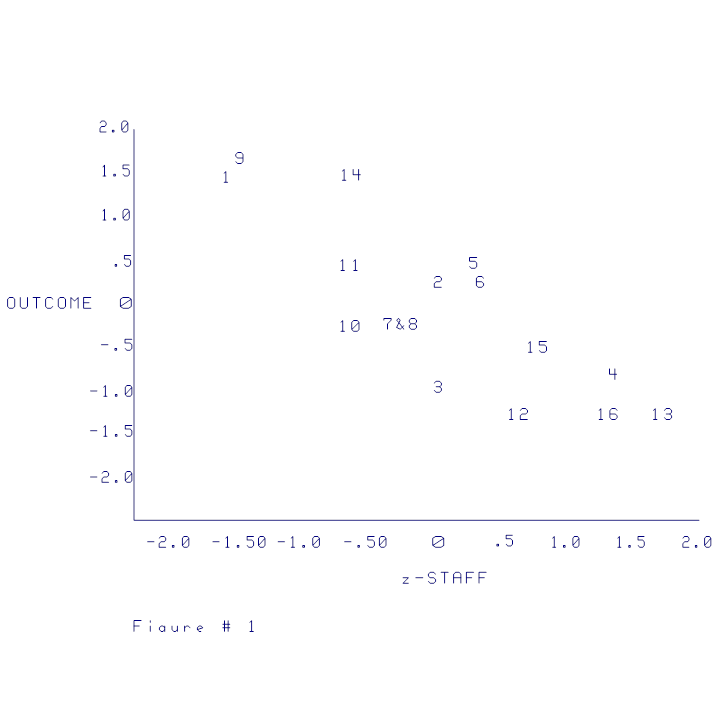
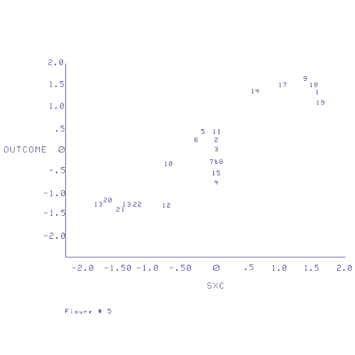
The scatterplots presented in Figures 1,
2, and 3 show how the reversal takes place and how to interpret its
meaning. Figure 1 shows the negative
relationship between the independent variable and the dependent variable. Figure 2 shows the positive relationship
between the adjusted variable and the dependent variable.
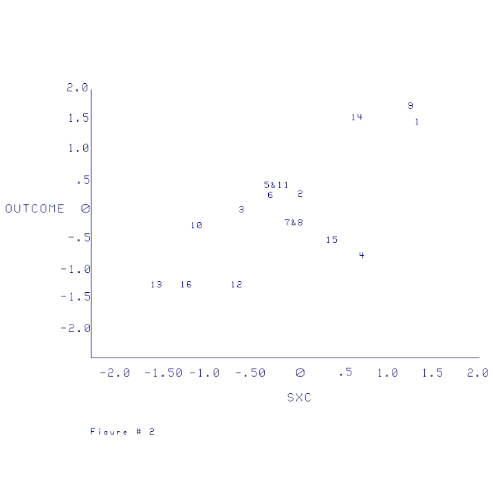
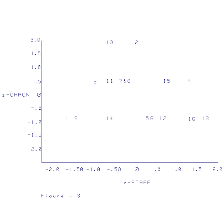
Figure 3 shows how the adjusted scores can
reflect treatment optimization and discrepancy.
The effects of multiplying the z‑ scores of the modifier variable
by the z‑scores of the independent variable are as follows. The adjusted score is positive (higher) when;
(1) treatment and chronicity are both high
(upper right
quadrant Fig. 3) or
(2) treatment and chronicity are both low
(lower left
quadrant Fig. 3)
These quadrants represent patients who
were well matched to the treatment.
Chronic patients who needed more treatment received more treatment and
acute patients who needed less treatment received less treatment. These adjusted scores reflect patients who
are matched to treatment with positive (high) scores. It should be noted that this matching (or
optimization) represents an hypothesis to be tested. The hypothesis is that chronic patients need
more treatment than acute patients in order to make equal outcome gains.
The adjusted score is negative (lower) when:
(3) treatment is low and chronicity is high
(upper left
quadrant Fig. 3) or
(4) treatment is high and chronicity is low
(lower right
quadrant Fig. 3)
These quadrants represent patients who
were mismatched to the treatment
according to the theory. Chronic
patients who needed more treatment received less and acute patients who needed
less treatment received more. The
adjusted scores reflect a mismatch in that the results are negative (low)
scores. The adjusted variable, then, is
an indicator of degree of optimization or matching (according to the
hypothesis): a high score represents optimization while a low
score represents a discrepancy. If this
adjusted score is positively related to outcome then the hypothesis that
chronic patients should receive more treatment is supported.
The scatterplots in Figures 1, 2, and 3
and the data in Table 1 show how the data in the example data fit the adjusted
scores. An acute patient (low
chronicity) receiving little treatment would obtain the high adjusted score, as
shown by cases 1, 9, and 14 in Figure 3.
Note that these cases are in the lower left hand quadrant of the
table. The z‑scores for these variables
are presented in Table 1. The z‑scores
for case 1 are ‑1.61 for treatment and ‑.88 for chronicity. The result of multiplying ‑1.61 by ‑.88
is 1.42 a positive score on the adjusted variable. Consequently, the score changed from a high
negative score on STAFF to a high positive score on the adjusted variable
(SXC). The same is true of cases 9 and
14. It can be noted on the change from
Fig 1 to Fig 2 that these cases change from negative to positive.
Cases 16 and 13 represent a mismatch change
for the adjusted score. Case 13 was
positive on treatment (z = 1.74) but negative on chronicity (z = ‑.88). The result is a negative adjusted score of ‑1.52
which indicates lack of optimal treatment according to the theory. Consequently, the cases in the upper left
quadrant of Figure 3 resulted in changing the positive staff scores to negative
adjusted scores.
This adjusted variable that represents
degree of optimization can now be correlated with outcome. If it correlates with outcome, it would
indicate that patients who got the appropriate amount of treatment got better
and patients who did not receive the optimal treatment did no get better. It indicates that patients who were matched
for treatment (chronic patients more treatment and acute patients less
treatment) obtained high positive outcomes and patients who were mismatched for
treatment obtained low or negative outcomes.
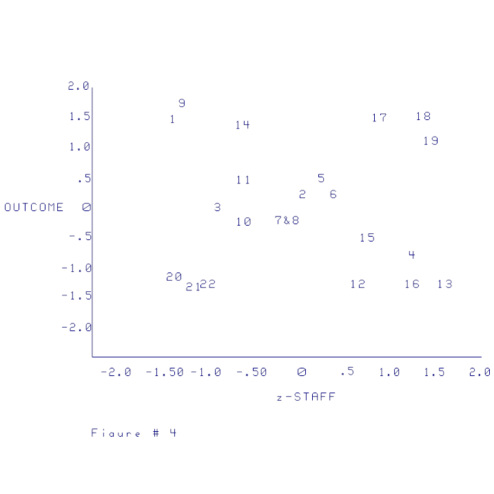
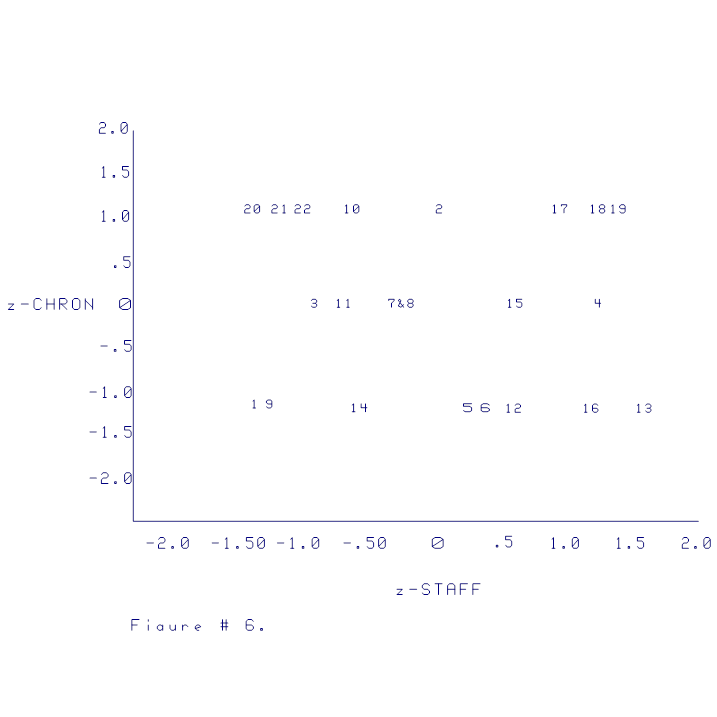
This interaction can take place also when
the original dependent variable correlates zero with the dependent variable. Six cases were arbitrarily added to the
original 16 cases to show this effect.
The data are found in Table 3, the resulting correlation matrix is in
Table 4, and scatterplots are in Figures 4, 5, and 6. The correlation matrix in Table 4 shows that
the relationship between the independent variable and the dependent variable is
.00 and the relationship between the adjusted variable and the dependent
variable is .91 thus demonstrating the it is not necessary for the original
independent variable to be negative.
_____________________________________________________________________
TABLE III. Data with 6 cases added to show
relationships.
┌────────────────────────────────────────────────────────────────────┐
│ OUTCOME STAFF
z‑STAFF CHRON z‑CHRON SXC
│
│
│
│ 1
1.42 3.3 ‑1.41 0
‑1.15 1.61 │
│ 2
.23 4.6 0.01 2
1.15 0.01
│
│ 3 ‑.00 3.8
‑0.86 1 0.00
0.00 │
│ 4 ‑.74 5.7
1.21 1 0.00
0.00 │
│ 5
.46 4.8 0.23 0
‑1.15 ‑0.26 │
│ 6
.23 4.9 0.34 0
‑1.15 ‑0.39 │
│ 7 ‑.28 4.4
‑0.21 1 0.00
0.00 │
│ 8 ‑.28 4.4
‑0.21 1 0.00
0.00 │
│ 9
1.65 3.4 ‑1.30 0
‑1.15 1.49 │
│ 10 ‑.28 4.1
‑0.53 2 1.15
‑0.61 │
│ 11
.46 4.1 ‑0.53 1
0.00 0.00 │
│ 12 ‑1.25 5.1
0.56 0 ‑1.15 ‑0.64 │
│ 13 ‑1.25 6.0
1.54 0 ‑1.15 ‑1.76 │
│ 14
1.42 4.1 ‑0.53 0
‑1.15 0.61 │
│ 15 ‑.51 5.2
0.67 1 0.00
0.00 │
│ 16 ‑1.25 5.7
1.21 0 ‑1.15 ‑1.39 │
│ 17
1.50 5.4 0.88 2
1.15 1.01 │
│ 18
1.50 5.8 1.32 2
1.15 1.51 │
│ 19
1.10 5.9 1.43 2
1.15 1.64 │
│ 20 ‑1.20 3.3
‑1.41 2 1.15
‑1.61 │
│ 21 ‑1.35 3.4
‑1.30 2 1.15
‑1.49 │
│ 22 ‑1.25 3.6
‑1.08 2 1.15
‑1.24 │
│
│
└────────────────────────────────────────────────────────────────────┘
A comparison of the two sets of data also
demonstrates the difference between the moderator variable and modifier
variable. As noted earlier the
definition of the modifier variable is defined differently than a moderator
variable (e.g., Ghiselli) in that a moderator variable must increase the
variance accounted for in a multiple regression. In the first example the modifier is reversed
from the dependent variable (in the first example) ‑ making a
considerable difference in interpretation.
Both relationships are significant in the opposite direction the added
variance, however, in the multiple regression only about 2% of the variance is
added in the multiple regression by the addition of the adjusted variable.
It can be noted in this second example
that the adjusted variable would add 80% variance beyond the independent
variable. So that in this instance the
test of the added variance in a multiple correlation would be an adequate test
of the variable. However, as seen in the
previous example if the relationship is reversed (the sign changed) then the
multiple regression may not detect this such a difference.
This raises the issue of how the test of
significance should be assessed. The
method of using multiple regression to the change by adding the adjusted
variable is not appropriate because it can be seen that a complete reversal if
direction without significance. One
possible method would be to test the
difference between rxy and ray. However, that would only test the interaction
and it is possible that rxy might negative while ray would be zero resulting in
a significant interaction. Even though
the difference is significant the zero correlation of ray indicates no
relationship between the modified variable and the independent variable.
Consequently, the following rules would
seem to apply: (1) if the signs are opposite the ray correlation could be
tested for significance beyond zero, and (2) if the signs are the same, then
the method of testing the additional variance beyond the independent variable
should be used.